
TLDR: There’s no official crosswalk between the ONET’s occupational taxonomy and ANZSCO, which is awkward, because Australian researchers use ONET data all the time. This post builds one, explains why you should be suspicious of relying on it and then suggests a better methodology is probably what was applied by the European Commission.
Update(s):
- A number of people reached out to me and said they developed their mapping to ANZSCO using propriety datasets, such as from job search data. Alas, these can’t be shared publicly.
- David Hood reached out to me and shared the mapping he used for his Covid-19 case rate analysis here (see ANZSCOMapping.xlsx). This was based on Figure.nz‘s mapping. Based on my cursory glance, it appears they’ve produced this by combining similar crosswalk pairs to the code below(?).
Background
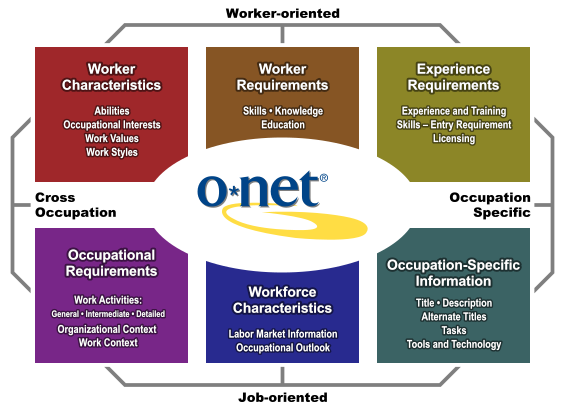
In 2025 I served as an adviser for a project to map occupational transition pathways in India. Although the work leveraged locally-sourced data and occupational profiles, the methodology leaned heavily on studies that use occupational profile data from the Occupational Information Network (O*NET). With the basic idea being that the viability of a transition pathway was in-part determined by how similar two jobs are (conditional on geography, wage rate differentials, education etc).
The Boring Part
I plan to write more about the interesting parts of this project in the future, but I need to start with the boring parts first: developing a crosswalk table between the O*NET-SOC taxonomy and national standards.
The Structure of ANZSCO
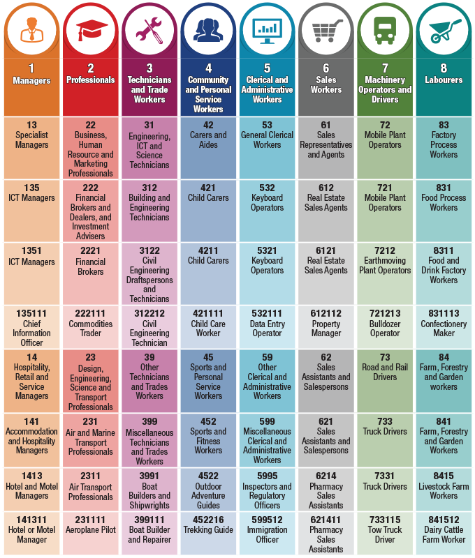
I’ll focus on developing a crosswalk / correspondence table between the O*NET-SOC and the Australian and New Zealand Standard Classification of Occupations (ANZSCO). This is both because I’ll use this crosswalk in a future post that uses this standard and as an “official” crosswalk doesn’t exist (despite Australian researchers frequently using the O*NET database).
Comparison between ANZSCO and ISCO-08
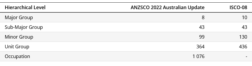
I suspect one reason official correspondence tables don’t exist already is that the OSCA is a new standard and that the O*NET SOC taxonomy doesn’t cleanly match to the ANZSCO or intermediate correspondence tables. In practice, this means the judgement of the analyst will be required to decide how to match one standard with the other so that it suits their use-case. For instance, if the research is on occupations in the Trucking industry it will be sensible to confirm the data you’re drawing on is being sensibly assigned.
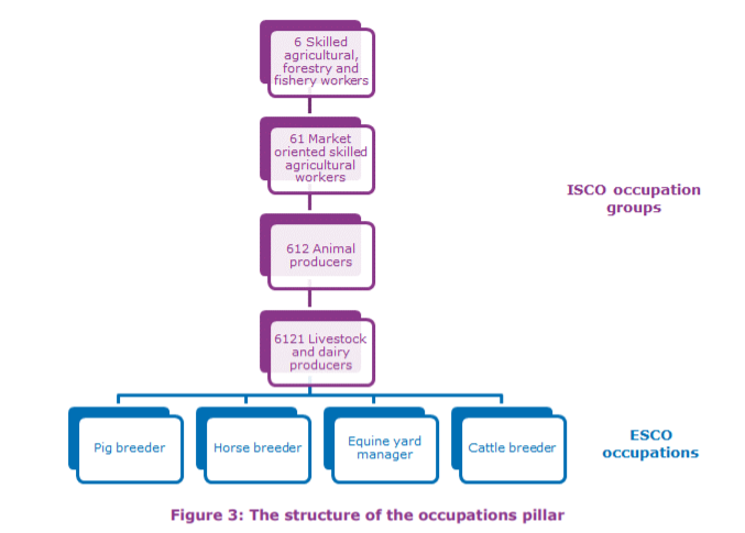
ISCO-08 and the European Skills, Competences, Qualifications and Occupations (ESCO) classification system
This problem isn’t exclusive to occupational correspondences. The same problems will often rear their head when trying to connect datasets that use different definitions for industries, administrative boundaries and/or products. In most cases the difficulty stems from each standard using a different approach for defining groups, which results in occupations being weirdly assigned at each step of creating a map between standards.
O*NET-SOC 2019 Taxonomy
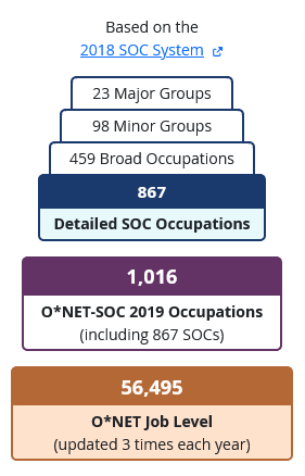
In the case of this post, the problems reared their head at every step from SOC to ANZSCO:
- From ANZSCO to OSCA: In most cases ANZSCO occupations have been assigned to one or more OSCA group, but there are cases where the opposite occurs too, such as Production Manager (Manufacturing), which has been assigned more than one ANZSCO grouping.
- From ISCO-08 (or ESCO) to OSCA: The bridge between the OSCA to ISCO suffers similar problems. However, because ISCO-08 groupings are only provided at the unit group level, in most cases OSCA occupations are bundled into large groups. However, the opposite also occurs too, with Engineering Technologist being assigned to several ISCO-08 groupings at the same time.
- From SOC to ISCO-08 (or ESCO): one of the best crosswalks directly maps occupations from the ESCO to the O*NET. Once again, these aren’t 1:1 matches,. For example, the ISCO/ESCO job Sports, recreation and cultural centre managers is assigned two jobs from the O*NET. While the O*NET occupation legislators is assigned to more than one distinct ISCO/ESCO occupation category.
The reason I mention this upfront is to make it clear the process is messy. And if I wasn’t intending to replicate research that uses ANZSCO in a future post I wouldn’t bother. But, I am, so I thought I should share my process (and pain) so other people can learn from my mistakes and re-purpose the approach in a way that suits their analysis.
Note: Because the Occupation Standard Classification for Australia (OSCA) is the modern successor of the ANZSCO, this crosswalk (and post) will have a short shelf-life.
Data: the correspondence tables used in this post are available here for the O*NET and here for the ABS. These were originally sourced from the O*NET and ABS on 21/8/2026.
How I used AI in this post: Because developing the correspondence table mainly requires data cleaning and joining occupational definitions, Claude was heavily leaned on to write the code for this post. The write up is more or less untouched by AI.
Project Setup
The code below sets the assumptions for importing correspondence tables and saving outputs.
|
1 2 3 4 5 6 7 8 9 10 11 12 13 14 15 16 17 18 19 20 21 22 23 24 25 26 27 28 29 30 31 32 33 34 35 36 37 38 39 40 41 42 43 44 45 46 47 48 49 50 51 52 53 54 55 56 57 58 59 60 61 62 63 64 65 66 67 68 69 70 71 72 73 74 75 76 77 78 79 80 |
library(tidyverse) library(readxl) library(janitor) ref_dir_data <- file.path(".", "Data") ref_dir_out <- file.path(".", "Outputs") ref_file_esco_to_soc <- file.path(ref_dir_data, "ESCO_to_ONET-SOC.xlsx") ref_file_osca_tables <- file.path(ref_dir_data, "OSCA_correspondence_tables_v2.xlsx") # Keep a SOC link only if this share of the ANZSCO unit group's detailed # occupations backs it. Set to 0 to keep everything. ref_min_pct_unit_support <- 50 #import the O*NET / ESCO crosstab dta_esco_soc_raw <- read_excel(ref_file_esco_to_soc, sheet = 1, skip = 3, col_types = "text") |> clean_names() |> filter(!is.na(esco_isco_code), !is.na(o_net_soc_2019_code)) |> transmute( esco_code = str_trim(esco_isco_code), # e.g. "8332.5" or "8332" esco_name = str_trim(esco_isco_title), isco_code = str_trim(str_extract(esco_isco_code, "^[^.]+")), isco_digits = str_length(isco_code), soc_code = str_trim(o_net_soc_2019_code), soc_name = str_trim(o_net_soc_2019_title), link_level = if_else(str_detect(esco_isco_code, "\\."), "esco_occupation", "isco_unit_group") ) # A few rows sit at ISCO MINOR group level (3 digits, e.g. "213"), which is # coarser than a unit group, so they cannot be placed and are dropped. dta_esco_soc_unitlevel <- dta_esco_soc_raw |> filter(isco_digits == 4) # ESCO maps some ISCO unit groups directly, and others only via the narrow # occupations inside them. tHEPrefer the direct mapping; fall back to the # occupation rows for the 84 groups that have none. lkp_isco_with_own_row <- dta_esco_soc_unitlevel |> filter(link_level == "isco_unit_group") |> pull(isco_code) |> unique() dta_esco_soc_kept <- dta_esco_soc_unitlevel |> filter(link_level == "isco_unit_group" | !(isco_code %in% lkp_isco_with_own_row)) # Table 8 is written OSCA -> ISCO; we travel it ISCO -> OSCA. Same pairs. dta_osca_to_isco <- read_excel( ref_file_osca_tables, sheet = "Table 8", col_names = c("osca_code", "osca_name", "isco_code", "match_flag", "isco_name"), col_types = "text", range = cell_limits(ul = c(6L, 1L), lr = c(NA_integer_, 5L)) ) |> # The last row is an ABS copyright line, not data. filter(!str_detect(coalesce(osca_code, ""), "Commonwealth")) |> fill(osca_code, osca_name, .direction = "down") |> filter(!is.na(isco_code)) |> # "xxxxxx" is the ABS marker for "no counterpart exists". filter(osca_code != "xxxxxx", isco_code != "xxxxxx") |> mutate(across(c(osca_code, isco_code), str_trim)) |> distinct(osca_code, osca_name, isco_code, isco_name) # Table 1 is written ANZSCO -> OSCA. dta_anzsco_to_osca <- read_excel( ref_file_osca_tables, sheet = "Table 1", col_names = c("anzsco_code", "anzsco_name", "osca_code", "match_flag", "osca_name"), col_types = "text", range = cell_limits(ul = c(6L, 1L), lr = c(NA_integer_, 5L)) ) |> filter(!str_detect(coalesce(anzsco_code, ""), "Commonwealth")) |> fill(anzsco_code, anzsco_name, .direction = "down") |> filter(!is.na(osca_code)) |> filter(anzsco_code != "xxxxxx", osca_code != "xxxxxx") |> mutate(across(c(anzsco_code, osca_code), str_trim)) |> distinct(anzsco_code, anzsco_name, osca_code) |> # ANZSCO codes are 6 digits (a detailed occupation). The first 4 are the unit # group, which is the level the O*NET analysis reports at. mutate(anzsco_unit_code = str_sub(anzsco_code, 1, 4)) |
Joins
The code below joins each correspondence pair sequentially. Because each mapping splits and merges occupational classifications differently, the unified crosswalk results isn’t a clean 1:1 correspondence. For this reason a better approach is likely to be matching occupational descriptions from either standard, such as was done by the European Commission for mapping the O*NET to ISCO-08, but I’ve already written the code so here we are…
|
1 2 3 4 5 6 7 8 9 10 11 12 13 14 15 16 17 18 19 20 21 |
# Start at the ESCO level of detail: one row per ESCO occupation and SOC code. dta_esco_x_soc <- dta_esco_soc_kept # COLLAPSE to the ISCO unit group. This is where the ESCO occupation codes and # names get dropped -- they cannot be carried further, because the ABS tables # are keyed on the ISCO unit group and not on ESCO. dta_isco_x_soc <- dta_esco_x_soc |> distinct(isco_code, soc_code, soc_name) dta_isco_x_soc_x_osca <- dta_isco_x_soc |> inner_join(dta_osca_to_isco, by = join_by(isco_code), relationship = "many-to-many") dta_isco_x_soc_x_osca_x_anzsco <- dta_isco_x_soc_x_osca |> inner_join(dta_anzsco_to_osca, by = join_by(osca_code), relationship = "many-to-many") dta_crosswalk_all_levels <- dta_isco_x_soc_x_osca_x_anzsco |> select(soc_code, soc_name, isco_code, isco_name, osca_code, osca_name, anzsco_code, anzsco_name, anzsco_unit_code) |> arrange(soc_code, isco_code, anzsco_code) |
Collapsing Occupations to the Unit-Group Level
Because the OSCA occupations are only mapped to the ISCO-08 unit-group (the first 4 digits of the code), the code below collapses the correspondence table to provide a listing of major SOC and ESCO occupations by unit group. As you’d expect, this results in a lot of granularity being lost.
|
1 2 3 4 5 6 7 8 9 10 11 12 13 14 15 16 17 18 19 20 21 22 23 24 25 26 27 28 29 30 31 32 33 34 35 36 37 38 39 40 41 42 |
lkp_anzsco_unit_detail <- dta_crosswalk_all_levels |> distinct(anzsco_unit_code, anzsco_code, anzsco_name) |> summarise( nmb_unit_occs = n_distinct(anzsco_code), # These files carry no ANZSCO unit group titles, only occupation titles, so # the lowest-numbered occupation stands in as the label. anzsco_unit_name = anzsco_name[order(anzsco_code)][1], .by = anzsco_unit_code ) # Advisory sanity check: do the ISCO major group (1st digit) and the SOC major # group (1st 2 digits) sit in compatible broad families? Some ESCO mappings are # simply poor, and this catches them. It has false positives, so it is reported # as a column and never filtered on. lkp_valid_major_group_pairs <- tribble( ~isco_major, ~soc_majors, "0", "55,33", # armed forces "1", "11", # managers "2", "13,15,17,19,21,23,25,27,29", # professionals "3", "13,15,17,19,21,25,29,31,33,49", # technicians "4", "41,43", # clerical "5", "31,33,35,37,39,41", # service and sales "6", "45", # agriculture "7", "47,49,51", # trades "8", "51,53", # plant and machine "9", "35,37,41,45,47,53" # elementary ) |> separate_longer_delim(soc_majors, delim = ",") |> rename(soc_major = soc_majors) |> mutate(broad_group_match = TRUE) rlt_crosswalk_by_unit_group <- dta_crosswalk_all_levels |> summarise(nmb_occ_support = n_distinct(anzsco_code), .by = c(soc_code, soc_name, isco_code, anzsco_unit_code)) |> left_join(lkp_anzsco_unit_detail, by = join_by(anzsco_unit_code)) |> mutate(pct_unit_support = round(100 * nmb_occ_support / nmb_unit_occs, 1), isco_major = str_sub(isco_code, 1, 1), soc_major = str_sub(soc_code, 1, 2)) |> left_join(lkp_valid_major_group_pairs, by = join_by(isco_major, soc_major)) |> mutate(broad_group_match = coalesce(broad_group_match, FALSE)) |> select(-isco_major, -soc_major) |> arrange(soc_code, anzsco_unit_code) |
Filtering out Poor Matches
The final step drops matches that are supported by a minority of occupations after joins. Each ANZSCO group holds several occupations and the joins match each of them to a SOC group separately. So, when more ANZSCO occupations are matched to the same SOC code within a unit group it’s assumed the match is stronger, while weaker matches are dropped and assumed to reflect the many quirks of trying to match definitions like this.
|
1 2 3 4 5 6 7 8 9 10 11 12 13 14 15 16 17 18 |
rlt_crosswalk_for_onet <- rlt_crosswalk_by_unit_group |> filter(pct_unit_support >= ref_min_pct_unit_support) |> summarise(isco_codes = paste(sort(unique(isco_code)), collapse = "; "), pct_unit_support = max(pct_unit_support), broad_group_match = any(broad_group_match), .by = c(anzsco_unit_code, anzsco_unit_name, soc_code, soc_name)) |> select(anzsco_code = anzsco_unit_code, label_4digit = anzsco_unit_name, soc = soc_code, soc_label = soc_name, isco_codes, pct_unit_support, broad_group_match) |> arrange(anzsco_code, soc) stopifnot( "Duplicate anzsco_code x soc rows would double-weight a SOC in the O*NET average" = nrow(rlt_crosswalk_for_onet) == nrow(distinct(rlt_crosswalk_for_onet, anzsco_code, soc)) ) |
Exploratory analysis
Claude produced a lot of exploratory analysis and checks after I harangued it and quizzed its analysis, but I think the summary below is the most useful. It essentially checks how many occupations from the source correspondence files remained in the unit-group mapping.
The TLDR: most of the O*NET occupations made it, despite the inconsistencies encountered along the way. On one level that’s a surprisingly good outcome, particularly given how naive the final mapping approach is. But it hides a few things that I’d worry about if using the table in my analysis: occupations being more likely to drop out in some categories more than others and SOC occupations landing in the wrong groups (which could result in drawing on incorrect data from the O*NET).
|
1 2 3 4 5 6 7 8 9 10 11 12 13 14 15 16 17 18 19 20 21 22 23 24 25 26 27 28 29 30 31 |
# The links behind the delivered table, taken at the level where isco_code is # still a single column. This is the same set of links as rlt_crosswalk_for_onet. dta_final_links <- rlt_crosswalk_by_unit_group |> filter(pct_unit_support >= ref_min_pct_unit_support) # Codes are lost at two different points, so both are reported. The joins are # inner joins, so a code with no counterpart drops out silently. The support # filter then removes more. OSCA is an intermediate hop and is not carried into # the final table at all, so it has no final count. rlt_codes_kept_vs_dropped <- tibble( classification = c("O*NET-SOC", "ISCO-08", "OSCA", "ANZSCO (unit group)"), nmb_in_source = c( n_distinct(dta_esco_soc_raw$soc_code), n_distinct(c(dta_esco_soc_unitlevel$isco_code, dta_osca_to_isco$isco_code)), n_distinct(c(dta_osca_to_isco$osca_code, dta_anzsco_to_osca$osca_code)), n_distinct(dta_anzsco_to_osca$anzsco_unit_code)), nmb_after_joins = c( n_distinct(dta_crosswalk_all_levels$soc_code), n_distinct(dta_crosswalk_all_levels$isco_code), n_distinct(dta_crosswalk_all_levels$osca_code), n_distinct(dta_crosswalk_all_levels$anzsco_unit_code)), nmb_in_final = c( n_distinct(dta_final_links$soc_code), n_distinct(dta_final_links$isco_code), NA_integer_, n_distinct(dta_final_links$anzsco_unit_code)) ) |> mutate(nmb_dropped = nmb_in_source - nmb_in_final, pct_kept = round(100 * nmb_in_final / nmb_in_source, 1)) rlt_codes_kept_vs_dropped |
Checking Final Crosswalk Coverage
The final code block below does a final check the coverage of the final mapping to determine how much information might have been lost by jumping between standards. In our case, our correspondence file is missing around 11 percent of jobs that were listed in the SOC to ESCO Correspondence table:
|
1 2 3 4 5 6 |
#check how many jobs in the original SOC to ESCO crosswalk exist in the final #correspondence #(a little under 90 percent) table(dta_esco_soc_raw$soc_code %in% rlt_crosswalk_for_onet$soc) |> prop.table() |> round(2) |
Output files
The final code block outputs the crosswalks.
|
1 2 3 4 5 6 7 8 9 |
ref_stamp <- format(Sys.Date(), "%y%m%d") if (!dir.exists(ref_dir_out)) dir.create(ref_dir_out) write_csv(dta_crosswalk_all_levels, file.path(ref_dir_out, paste0(ref_stamp, " - crosswalk_full.csv"))) write_csv(rlt_crosswalk_by_unit_group, file.path(ref_dir_out, paste0(ref_stamp, " - crosswalk_unit.csv"))) write_csv(rlt_crosswalk_for_onet, file.path(ref_dir_out, paste0(ref_stamp, " - crosswalk_for_onet.csv"))) |
Summing up
Because the main point of this post is to produce a correspondence table for a future post, I’m not going to split hairs about the assignment. However, if you’re intending to use the crosswalks for something more rigorous, I hope this post demonstrates clearly why you should.
A few things I’d check:
- What was dropped and is it valuable to your analysis. This approach lost a little over ten per cent of jobs from the original SOC to ESCO mapping, which may be important if these gaps cover occupations your analysis relies on and/or risks biasing your results.
- Confirm assignments for occupations your analysis relies on. For me, it’s truck drivers as the next post replicates analysis that looks at occupational paths for that group.
- Validate assignments / groupings. Particularly for above, but the approach I’ve used is naive insofar as I’ve just joined each table together and used a simple filtering mechanism for dropping obvious cases. However, having done this makes me even more convinced that a simple comparison of job titles or descriptions would be easier to justify (like the European Commission’s methodology).
Which is perhaps something I’ll do in a future post, but for now I’d just say that if you have a better approach, or want to point out the problems with mine, please get in touch. I wrote this up in an afternoon: this isn’t mean to be a master work. So, I’ll happily link to better approaches and make corrections to avoid leading others astray.