
TLDR: Weighted by population, the rule of law has slipped globally since 1996. India and the United States contributed a large part to this decline, while China’s net impact was negligible thanks to a recovery from the mid 00’s. Countries with a stronger rule of law tend to be wealthier, and those where it improved were more likely to grow faster, but there are plenty of exceptions to the rule, with China experiencing higher growth than might be expected from changes in its rule of law score, alongside Armenia, Bosnia and Herzegovina, Guyana and Myanmar.
How AI was used: AI was used to write the first draft of analysis included in this post. I then collaborated with AI to refine the post until it resembled what I had in mind: the majority of writing is therefore my own. AI also was used to put the post in a format compatible with WordPress.
Background
One of the reasons consulting suits me is that it provides me with an almost unlimited number of rabbit holes to get lost in. One such example that came up in 2025, was a project exploring the links between economic growth and the rule of law for the Bingham Centre for the Rule of Law and the Law Society of England and Wales. If you’re interested in exploring this further, I’d recommend Dr Lopez-Gomez’s literature review, which was a key outcome of the project.
This is the fourth post in my series on the rule of law (see earlier posts: 1, 2 and 3), with previous posts intended to demonstrate themes that this and future posts rely on, including that:
- The Worldwide Governance Indicator’s (WGI) Rule of Law index provides a reliable proxy for the World Justice Project’s (WJP) measure (with greater coverage over a longer period); and
- It’s probably not a good idea to solely use pairwise relationships for exploring how the rule of law interacts with other outcomes as these things are hard to measure, co-determined and probably operate within an interdependent system of institutions.
Four themes
Although I had grander plans when I first started drafting this post, I’ve scaled back my ambition to focus on four themes that provide useful context for future posts:
- Globally, the rule of law has deteriorated since the mid 90s.
- Countries with stronger rule of law are wealthier.
- Countries that improve their rule of law tend to grow faster.
- But, the rule of law isn’t a necessary or sufficient condition for economic growth.
Here be dragons
To avoid the need for weasel words and vague descriptors it’s worth remembering that cross-country analysis is a minefield:
- Institutions like the rule of law (etc) are hard to define and measure: Institutions are the rules, norms and conventions that shape, constrain and guide human behaviour and interactions. Institutions can run from the grand rules and expectations that ensure peaceful democratic transitions after an election to the mundane social norm that ensures Bill from Accounting doesn’t microwave his tuna salad at lunch. Whether the former is more important than the latter is a matter of taste, but being all encompassing, interdependent and hard to define also makes institutions difficult to measure. This is particularly true for perception-based measures as someone asked how well the rule of law works is likely to be thinking about democracy, accountability and government effectiveness too, while potentially making qualitative judgements that lean towards accepted Western models of governance.
- Interesting things tend to be correlated with one another: As institutions like the rule of law operate within an interdependent system (see last post), everything tends to be correlated with one another whether or not they are causally related. Economic growth probably depends on the quality of a country’s legal system, but the legal system itself likely also depends on economic growth too as it influences the resourcing available for government to invest in it. This makes it difficult to talk about the rule of law as a discrete characteristic independent of other institutions.
- National statistics obscure the relationships that matter: Cross-country statistics are not always representative of specific actors or the underlying causal mechanisms that we’re interested in. For instance, economic and social relationships sometimes transcend the nation-state (the unit of focus for cross-country analysis).
- Institutions are sticky and slow moving: We consider a time series of data running from 1996 to 2023, which is just short of three decades. Although this might feel long-run enough, leading studies in the field cover much longer periods e.g. 100+ years (see 1 and 2). In practical terms, this might mean that the strength and direction of relationships examined here might not generalise over longer periods.
But, I haven’t picked the themes covered here by accident: each of them tells a story supported by the literature, which I’ve done my best to cite throughout.
Project setup
Data
The rule of law measure is the Rule of Law dimension of the World Bank’s WGI, 2025 release, which covers 1996 to 2024.1 The WGI’s RoL attempts to measure the quality of contract enforcement, property rights, the police, the courts and the likelihood of crime and violence. The WGI’s measure has been selected on the basis of it covering a larger number of countries over a longer period. Earlier posts in the series also indicated it provides a reliable proxy for the WJP’s more comprehensive RoL measure. The data can be downloaded here.
Statistical measures, namely GDP per capita (PPP), GDP per capita growth, population and oil and gas rents, along with each country’s World Bank region, have been drawn from the World Development Indicators via the wbstats package. They were downloaded once, on 22 October 2026, and saved, so the results don’t change when the World Bank revises its figures. A snapshot of the data used here can be downloaded here.
Country income classifications were the earliest classifications available from the World Bank’s historical classification data (available here).
Pacific island small states are the World Bank’s group of that name, taken from its current country classification file (CLASS.xlsx, downloaded on 7 November 2026 from the same page).
Access to the sea, as the share of each country’s population living within 100 km of a coast or a navigable river, and the malaria index came from the geography dataset of Gallup, Sachs and Mellinger,2 downloaded on 7 November 2026 from RePEc.
The four code chunks below are used for loading libraries, specifying key assumptions, and importing and joining the data.
Code: setup
The code below loads the libraries, sets key assumptions and defines standard chart styles and labels for the rest of the post.
|
1 2 3 4 5 6 7 8 9 10 11 12 13 14 15 16 17 18 19 20 21 22 23 24 25 26 27 28 29 30 31 32 33 34 35 36 37 38 39 40 41 42 43 44 45 46 47 48 49 50 51 52 53 54 55 56 57 58 59 60 61 62 63 64 65 66 67 68 69 70 71 72 73 74 75 76 77 78 79 80 81 82 83 84 85 86 87 88 89 90 91 92 93 94 95 96 97 |
# load the packages we'll need library(tidyverse) library(readxl) library(janitor) library(ggrepel) #file paths ref_path <- list( wgi = file.path("Data", "wgidataset_with_sourcedata-2025.xlsx"), income_history = file.path("Data", "OGHIST_2026_10_08.xlsx"), # World Bank historical income groups wdi = file.path("Data", "261022 - wdi_indicators.csv"), # WDI indicators and regions pacific = file.path("Data", "261107 - pacific_island_small_states.csv") # World Bank Pacific island small states ) #years covered ref_year <- list( start = 1996, # the first WGI year end = 2023, # the last year with near-complete WDI coverage for most series rents_window = 2019:2023 # the last five years, averaged for oil and gas rents, which swing with prices ) #cut-offs that define samples and groups ref_cutoff <- list( min_growth_years = 20, # countries with fewer years of growth data are dropped large_producer_rents_pct = 10, # oil and gas rents above this share of GDP mark a large producer min_group_countries = 5, # region and income groups with fewer countries are left off the correlation chart outlier_sd = 2 # countries further than this many standard deviations above the line are named on the growth chart ) #WDI indicators: short name = World Bank code ref_wdi_indicators <- c( econ_gdppc_ppp = "NY.GDP.PCAP.PP.KD", # GDP per capita, PPP, constant international $ econ_gdppc_growth_pct = "NY.GDP.PCAP.KD.ZG", # GDP per capita growth, annual % pop_tot_nmb = "SP.POP.TOTL", # population res_oil_rents_pct = "NY.GDP.PETR.RT.ZS", # oil rents, % of GDP res_gas_rents_pct = "NY.GDP.NGAS.RT.ZS" # natural gas rents, % of GDP ) #colours (from my site palette), set once for every chart ref_col <- list( navy = "#0C1446", # titles and strip labels charcoal = "#2B2E45", # body text grey = "#73768C", # axis labels, captions, annotations grey_light = "#C7CBD8", # background points and context grey_pale = "#E2E8F0", # gridlines and zero lines blue = "#2740DA", # the series the chart is about red = "#922C40", # decline orange = "#DC9750", # a second group shown beside the blue one green = "#16AF8E" # improvement ) #red and green always mean decline and improvement; the four hues in order for charts with several groups ref_col$direction <- c(Decline = ref_col$red, Improvement = ref_col$green) ref_col$series <- c(ref_col$blue, ref_col$red, ref_col$orange, ref_col$green) #chart text: the source caption, how to read a WGI axis, and the large producer legend # WGI scores run from about -2.5 to +2.5, centred on the average country. # Arrows turn with the text on a vertical axis, so vertical axes get words instead. ref_lab <- list( caption = "Source: Worldwide Governance Indicators (2025); World Development Indicators.", axis_score = "← weaker 0 = average country stronger →", axis_score_vertical = "higher = stronger; 0 = average country", axis_change = "← worsened 0 = no change improved →", large_producers = paste0("Oil and gas rents above ", ref_cutoff$large_producer_rents_pct, "% of GDP"), clear_of_error = "* The change is larger than its 90% measurement band, which lies wholly on one side of zero.", income_start = "Income groups are each country's earliest World Bank classification (for most, based on 1987 income), not its current one." ) #series colours for charts with up to four groups options(ggplot2.discrete.colour = ref_col$series, ggplot2.discrete.fill = ref_col$series) # Open Sans needs to be installed; ragg (set in the YAML) picks it up. theme_set( theme_minimal(base_size = 11, base_family = "Open Sans") + theme(text = element_text(colour = ref_col$charcoal), axis.text = element_text(colour = ref_col$grey), axis.title = element_text(size = rel(0.9)), axis.title.x = element_text(margin = margin(t = 8)), axis.title.y = element_text(margin = margin(r = 8)), panel.grid.minor = element_blank(), panel.grid.major.x = element_blank(), panel.grid.major.y = element_line(colour = ref_col$grey_pale, linewidth = 0.4), strip.text = element_text(colour = ref_col$navy, face = "bold", hjust = 0), legend.position = "top", legend.justification = "left", legend.title = element_blank(), plot.title = element_text(colour = ref_col$navy, face = "bold", size = rel(1.15)), plot.subtitle = element_text(colour = ref_col$grey, margin = margin(b = 10)), plot.title.position = "plot", plot.caption = element_text(colour = ref_col$grey, face = "italic", size = rel(0.75), hjust = 0), plot.caption.position = "plot", plot.margin = margin(10, 15, 10, 10)) ) update_geom_defaults("text", list(family = "Open Sans", colour = ref_col$charcoal)) |
Importing data
Code: import-wgi
The code below imports the WGI and recodes countries so they align with the World Bank data.
|
1 2 3 4 5 6 7 8 9 10 11 12 13 14 15 16 17 18 19 20 21 |
# Read the Rule of Law sheet. The sheet has one unnamed column; "unique_quiet" # gives it a name without printing a message. dta_wgi_rol <- read_excel(ref_path$wgi, sheet = "rl", .name_repair = "unique_quiet") |> clean_names() # Keep the columns we need, with shorter names. Missing estimates may be # stored as text (such as ".."), so the scores are converted to numbers. dta_wgi_rol <- dta_wgi_rol |> mutate(year = as.integer(year), wgi_rol = as.numeric(governance_estimate_approx_2_5_to_2_5), wgi_rol_se = as.numeric(standard_error_estimate)) |> select(iso3c = economy_code, country = economy_name, year, wgi_rol, wgi_rol_se) # Older WGI releases used a few codes that are not ISO codes. This lookup # gives the ISO code for each one. lkp_iso_fixes <- c(ROM = "ROU", ZAR = "COD", TMP = "TLS", ADO = "AND", KSV = "XKX", WBG = "PSE") # Swap in the ISO code where the lookup has one; otherwise keep the code as it is dta_wgi_rol <- dta_wgi_rol |> mutate(iso3c = coalesce(unname(lkp_iso_fixes[iso3c]), iso3c)) |
Code: import-wdi
The code below imports the WDI data and the World Bank’s historical income classifications.
Each country is grouped by its earliest World Bank income classification to avoid the groups directly mirroring rule of law scores i.e. due to simultaneity between economic growth and the rule of law. This isn’t a perfect solution, but will have to suffice in the absence of an instrument.
|
1 2 3 4 5 6 7 8 9 10 11 12 13 14 15 16 17 18 19 20 21 22 23 24 25 26 27 28 29 30 31 32 33 34 35 36 37 38 39 40 41 42 43 44 45 46 47 48 49 50 51 52 53 54 55 56 57 58 59 60 61 62 63 64 |
# WDI indicators and World Bank regions, downloaded on 22 October 2026 with # wbstats::wb_data(indicator = ref_wdi_indicators, start_date = 1996, end_date = 2023), # and each country's region from wbstats::wb_countries(), with aggregates such as # "World" dropped dta_wdi <- read_csv(ref_path$wdi, show_col_types = FALSE) |> select(iso3c, country, region, year, all_of(names(ref_wdi_indicators))) |> mutate(year = as.integer(year)) # Income group names: World Bank code = full name, and full name = short name for charts lkp_income <- list( full = c(L = "Low income", LM = "Lower middle income", UM = "Upper middle income", H = "High income"), short = c("Low income" = "Low", "Lower middle income" = "Lower middle", "Upper middle income" = "Upper middle", "High income" = "High") ) # The World Bank's historical income classifications. The fiscal years (FY89 # to FY27) are in row 5, so the four title rows above it are skipped. Every # column is read as text, because the codes are letters. The first column # holds the country code. lkp_income_start <- read_excel(ref_path$income_history, sheet = "Country Analytical History", skip = 4, col_types = "text", .name_repair = "unique_quiet") |> rename(iso3c = 1) # Keep the country rows only. This drops the row of calendar years under the # fiscal years, and the notes at the foot of the sheet. lkp_income_start <- lkp_income_start |> filter(str_detect(iso3c, "^[A-Z]{3}$")) # Reshape to one line per country and fiscal year lkp_income_start <- lkp_income_start |> pivot_longer(starts_with("FY"), names_to = "fiscal_year", values_to = "income_code") # Keep the years in which a country was classified. ".." means not classified # that year. "LM*" is Yemen with a footnote, so the asterisk is removed first. lkp_income_start <- lkp_income_start |> mutate(income_code = str_remove(income_code, "\\*")) |> filter(income_code %in% names(lkp_income$full)) # Turn the fiscal year into a number: FY89 to FY99 are 1989 to 1999, and FY00 # onwards are 2000 onwards lkp_income_start <- lkp_income_start |> mutate(fiscal_year = as.integer(str_remove(fiscal_year, "FY")), fiscal_year = if_else(fiscal_year >= 80, 1900L + fiscal_year, 2000L + fiscal_year)) # Keep each country's earliest classification: slice_min() keeps the line with # the smallest fiscal year for each country lkp_income_start <- lkp_income_start |> slice_min(fiscal_year, n = 1, with_ties = FALSE, by = iso3c) # The columns used in the rest of the post: the income group's full name, the # fiscal year it comes from, and a simpler split of high income against # everyone else, used in later charts lkp_income_start <- lkp_income_start |> mutate(econ_income_start = unname(lkp_income$full[income_code]), econ_income_start_fy = fiscal_year, econ_hic_start = if_else(econ_income_start == "High income", "High income", "Low & middle income")) |> select(iso3c, econ_income_start, econ_income_start_fy, econ_hic_start) # Number of countries in each starting income group count(lkp_income_start, econ_income_start, econ_hic_start) |
# A tibble: 4 × 3
  econ_income_start   econ_hic_start          n
  <chr>               <chr>               <int>
1 High income         High income            54
2 Low income          Low & middle income    51
3 Lower middle income Low & middle income    78
4 Upper middle income Low & middle income    40
Code: join
The code below joins WGI and WDI datasets into a single panel dataset. Countries that failed to join are listed, as are countries scored in 1996 whose first income classification came later.
|
1 2 3 4 5 6 7 8 9 10 11 12 13 14 15 16 |
# Add the WGI scores to the WDI data, matching on country code and year. The # WDI data already has the country names, so the WGI's are dropped. dta_panel <- dta_wdi |> left_join(select(dta_wgi_rol, -country), by = join_by(iso3c, year), relationship = "one-to-one") # Add each country's starting income group dta_panel <- dta_panel |> left_join(lkp_income_start, by = join_by(iso3c), relationship = "many-to-one") # WGI economies with no match in the WDI data. Most are territories, such as # Jersey, or economies the World Bank doesn't cover, such as Taiwan. chk_wgi_unmatched <- dta_wgi_rol |> distinct(iso3c, country) |> anti_join(distinct(dta_panel, iso3c), by = join_by(iso3c)) chk_wgi_unmatched |
# A tibble: 9 × 2
  iso3c country
  <chr> <chr>
1 GUF   French Guiana
2 MTQ   Martinique
3 TWN   Taiwan, China
4 AIA   Anguilla
5 ANT   Netherlands Antilles (former)
6 REU   Réunion
7 COK   Cook Islands
8 NIU   Niue
9 JEY   Jersey, Channel Islands
|
1 2 3 4 5 6 7 |
# Countries scored in 1996 whose first income classification came after 1996 chk_income_late <- dta_panel |> filter(year == ref_year$start, !is.na(wgi_rol)) |> filter(is.na(econ_income_start) | econ_income_start_fy > ref_year$start) |> select(iso3c, country, econ_income_start, econ_income_start_fy) chk_income_late |
# A tibble: 4 × 4
  iso3c country econ_income_start   econ_income_start_fy
  <chr> <chr>   <chr>                              <int>
1 NRU   Naoero  High income                         2017
2 PLW   Palau   Upper middle income                 1998
3 SRB   Serbia  Upper middle income                 2008
4 TUV   Tuvalu  Lower middle income                 2011
Global rule of law trends
To get a sense how the rule of law has changed, the code block below calculates the average rule of law score since 1996 across countries. Both unweighted and population-weighted scores are calculated, with the latter indicating how the rule of law has changed for the average person.
Note: Revisions to the WGI’s methodology in 2025 improve the ability for scores to be compared over time (see the World Bank’s methodology note, cited in the Data section above).
Code: population-weighted-trends
The code below calculates the global unweighted and weighted rule of law score. Only countries with WGI scores in the first year are included so the number of countries remain fixed.
|
1 2 3 4 5 6 7 8 9 10 11 12 13 14 15 16 17 18 19 20 21 22 23 24 25 26 27 28 29 30 31 32 33 34 35 36 37 38 39 40 41 |
# The countries with a score in 1996. Only these countries are kept, so the # same countries are averaged in every year. ref_countries_1996 <- dta_panel |> filter(year == ref_year$start, !is.na(wgi_rol)) |> pull(iso3c) # Keep those countries, in every year where they have a score, a standard # error, a population and a starting income group dta_panel_1996 <- dta_panel |> filter(iso3c %in% ref_countries_1996, !is.na(wgi_rol), !is.na(wgi_rol_se), !is.na(pop_tot_nmb), !is.na(econ_income_start)) # Order the income groups from poorest to richest (by the median GDP per # capita of each group), so charts list them in that order dta_panel_1996 <- dta_panel_1996 |> mutate(econ_income_start = fct_reorder(econ_income_start, econ_gdppc_ppp, .fun = median, .na_rm = TRUE)) # The world average in each year, weighted by population and unweighted. # Each standard error combines the WGI's country standard errors using the # same weights as the average. This assumes the measurement errors of # different countries are independent of one another. sum_rol_world_avg <- dta_panel_1996 |> summarise( wgi_rol_popw = weighted.mean(wgi_rol, w = pop_tot_nmb), wgi_rol_unw = mean(wgi_rol), wgi_rol_popw_se = sqrt(sum((pop_tot_nmb / sum(pop_tot_nmb))^2 * wgi_rol_se^2)), wgi_rol_unw_se = sqrt(sum(wgi_rol_se^2)) / n(), nmb_countries = n(), .by = year) |> arrange(year) # Change in the weighted average since 1996 sum_rol_world_avg <- sum_rol_world_avg |> mutate(wgi_rol_popw_change = wgi_rol_popw - wgi_rol_popw[year == ref_year$start]) # The change from 1996 to 2023, quoted in the text below sum_rol_world_change <- sum_rol_world_avg$wgi_rol_popw_change[sum_rol_world_avg$year == ref_year$end] |
The rule of law has declined globally
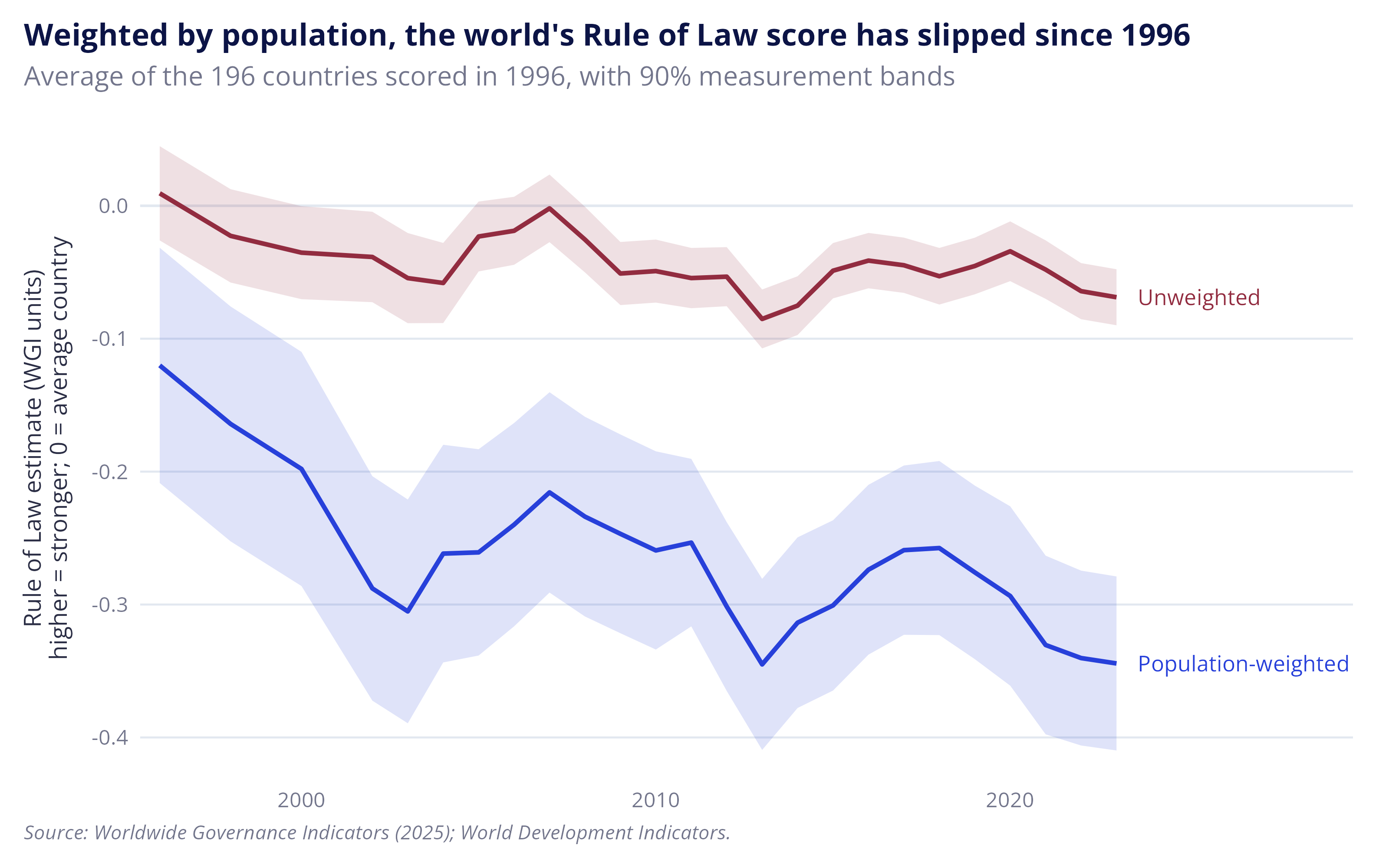
The chart below presents weighted and unweighted rule of law scores since 1996. Unweighted scores can be thought of as how the rule of law has changed for the average country, while the weighted scores are intended to show how it has changed for the average person. In both cases the rule of law appears to have declined globally, although the declines in unweighted scores only just clear the measurement error bands.
Note: Shaded bands are based on the standard errors provided by the WGI and can be thought of as margins of error. In their note on analytical issues with the WGI, Kaufmann, Kraay and Mastruzzi suggest that overlapping intervals can be thought of as a conservative test for whether two scores are the same.3 And while the generalized declines might be cause for alarm, the population-weighted fall of 0.22 is smaller than the 0.31 difference in scores between Denmark and New Zealand in 2023. This doesn’t mean that the changes aren’t significant from a governance standpoint, but just that the scale of these declines doesn’t necessarily point to the world becoming lawless.
Figure: World Rule of Law, population-weighted and unweighted, 1996–2023
Code: plot-world-trend
The code below produces a plot with the weighted and unweighted rule of law score since 1996. The shaded bands are based on 90 percent margins of errors provided by the WGI. The contributions to the average world score change is also estimated in dta_country_contrib, and the five most populous countries are picked out for the text and charts below.
|
1 2 3 4 5 6 7 8 9 10 11 12 13 14 15 16 17 18 19 20 21 22 23 24 25 26 27 28 29 30 |
# Stack the two averages into one table, one under the other, so each can be # drawn as its own line sum_plt_rol_world <- bind_rows( sum_rol_world_avg |> select(year, wgi_rol = wgi_rol_popw, wgi_rol_se = wgi_rol_popw_se) |> mutate(measure = "Population-weighted"), sum_rol_world_avg |> select(year, wgi_rol = wgi_rol_unw, wgi_rol_se = wgi_rol_unw_se) |> mutate(measure = "Unweighted") ) plt_rol_world_trend <- sum_plt_rol_world |> ggplot(aes(x = year, y = wgi_rol, colour = measure, fill = measure)) + geom_hline(yintercept = 0, colour = ref_col$grey_pale) + # 90% band: 1.645 standard errors either side of the average geom_ribbon(aes(ymin = wgi_rol - 1.645 * wgi_rol_se, ymax = wgi_rol + 1.645 * wgi_rol_se), colour = NA, alpha = 0.15) + geom_line(linewidth = 0.9) + geom_text(data = filter(sum_plt_rol_world, year == max(year)), aes(label = measure), hjust = 0, nudge_x = 0.6, size = 3.2) + scale_x_continuous(expand = expansion(mult = c(0.02, 0.22))) + theme(legend.position = "none") + labs(title = "Weighted by population, the world's Rule of Law score has slipped since 1996", subtitle = paste0("Average of the ", sum_rol_world_avg$nmb_countries[1], " countries scored in 1996, with 90% measurement bands"), x = NULL, y = paste0("Rule of Law estimate (WGI units)\n", ref_lab$axis_score_vertical), caption = ref_lab$caption) plt_rol_world_trend |
|
1 2 3 4 5 6 7 8 9 10 11 12 13 14 15 16 17 18 19 20 21 22 23 24 25 26 27 28 29 30 31 32 33 34 35 36 37 38 39 40 41 42 43 44 45 |
# How much each country added to, or took away from, the change in the # weighted world average. The weighted average in a year is the sum, across # countries, of population share x score. So a country's contribution to the # change is its share x score in 2023 less its share x score in 1996, and the # contributions add up to the change in the world line exactly. # Step 1: each country's share of the total population in 1996 and in 2023 dta_country_contrib <- dta_panel_1996 |> filter(year %in% c(ref_year$start, ref_year$end)) |> mutate(pop_share = pop_tot_nmb / sum(pop_tot_nmb), .by = year) |> mutate(period = if_else(year == ref_year$start, "start", "end")) |> select(iso3c, country, period, pop_share, wgi_rol, wgi_rol_se) # Step 2: put the two years side by side, one line per country, with the # columns pop_share_start, pop_share_end, wgi_rol_start, wgi_rol_end, # wgi_rol_se_start and wgi_rol_se_end dta_country_contrib <- dta_country_contrib |> pivot_wider(names_from = period, values_from = c(pop_share, wgi_rol, wgi_rol_se)) # Step 3: each country's contribution, and its change in score dta_country_contrib <- dta_country_contrib |> mutate(contrib = pop_share_end * wgi_rol_end - pop_share_start * wgi_rol_start, wgi_rol_change = wgi_rol_end - wgi_rol_start) # The five most populous countries in 2023, quoted in the text below and # charted in the next chunk dta_most_populous <- dta_country_contrib |> slice_max(pop_share_end, n = 5) # Is each change clear of measurement error? The standard error of the change # combines the 1996 and 2023 errors, treating them as independent, as for the # region and income groups below. A change is clear when its whole 90% band # (1.645 standard errors either side) lies on one side of zero. dta_most_populous <- dta_most_populous |> mutate(wgi_rol_change_se = sqrt(wgi_rol_se_start^2 + wgi_rol_se_end^2), clear_of_error = abs(wgi_rol_change) > 1.645 * wgi_rol_change_se) dta_most_populous <- dta_most_populous |> mutate(direction = if_else(wgi_rol_change < 0, "Decline", "Improvement"), # the axis label, for example "India (18% of population)", with an # asterisk after the name when the change is clear of measurement error country_label = sprintf("%s%s (%.0f%% of population)", country, if_else(clear_of_error, "*", ""), pop_share_end * 100), # order the labels by population, so the largest is at the top of the chart country_label = fct_reorder(country_label, pop_share_end)) |
India was a key driver of global declines in the rule of law
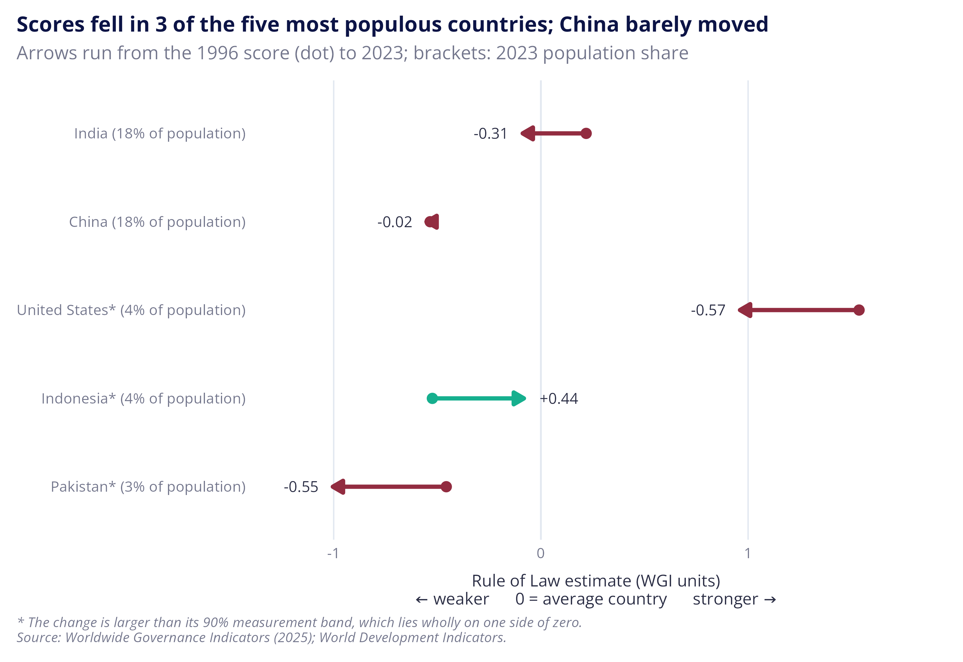
Population-weighted average rule of law scores mean more populous countries with larger score changes drive the global average. The code below explores this by looking at the source of declines, with a focus on the five most populated countries (accounting for 46% of world population).
The answer is mixed, with India, the United States and Pakistan experiencing declines, Indonesia an improvement and China showing next to no net change. Although India experienced smaller declines relative to the United States and Pakistan, its larger population made it a key driver of declines in the global weighted average rule of law score.
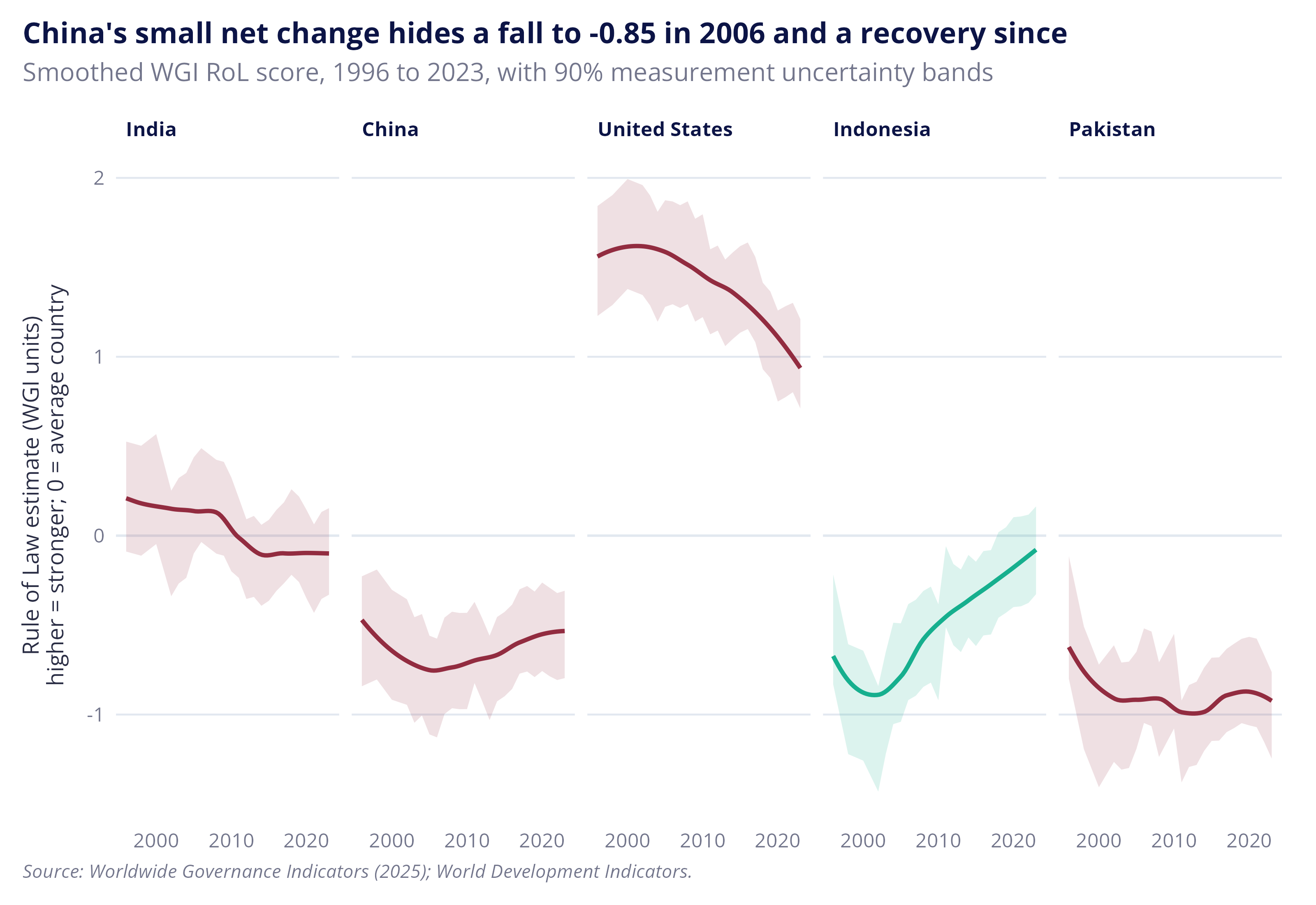
When each country’s score is viewed individually, the trends aren’t as clear cut. For instance, although India’s score has declined over the period, the change is within the bounds for measurement error, making it possible that score differences come down to measurement error rather than tangible changes in institutional quality (which is also true for China). On the other hand, the trends exhibited by the United States and Indonesia are large enough to point to real changes over the period: a decline for the former and improvement for the latter.
Figures: Rule of Law in the five most populous countries, 1996 and 2023, and in every year between
Code: world-trend-contributions
The rule of law scores for the five most populous countries: China, India, Indonesia, Pakistan and the United States are then visualized. The first plot shows the change in the WGI RoL score between 1996 and 2023, while the second plot shows how each country’s score has evolved over time, as a smoothed line with uncertainty bands.
|
1 2 3 4 5 6 7 8 9 10 11 12 13 14 15 16 17 18 19 20 21 22 23 24 25 26 27 28 29 30 31 32 33 34 |
# For the chart title: the country that moved least, and how many of the other # four declined. The least-changed country is left out of the count, so the # title doesn't count it as a fall and also say it barely moved. dta_populous_least_change <- slice_min(dta_most_populous, abs(wgi_rol_change), n = 1) sum_populous_nmb_fell <- sum(dta_most_populous$direction == "Decline" & dta_most_populous$iso3c != dta_populous_least_change$iso3c) plt_populous_change <- dta_most_populous |> ggplot(aes(y = country_label)) + geom_vline(xintercept = 0, colour = ref_col$grey_pale) + # each arrow runs from the country's 1996 score (dot) to its 2023 score; # the dot takes the arrow's colour geom_point(aes(x = wgi_rol_start, colour = direction), size = 2.5) + geom_segment(aes(x = wgi_rol_start, xend = wgi_rol_end, yend = country_label, colour = direction), arrow = arrow(length = unit(0.25, "cm"), type = "closed"), linewidth = 1.2) + # the change is printed beside the arrowhead, on the side it moved towards geom_text(aes(x = wgi_rol_end, label = sprintf("%+.2f", wgi_rol_change), hjust = if_else(direction == "Decline", 1.4, -0.4)), size = 3.2) + scale_colour_manual(values = ref_col$direction) + scale_x_continuous(expand = expansion(mult = 0.15)) + theme(legend.position = "none", panel.grid.major.y = element_blank(), panel.grid.major.x = element_line(colour = ref_col$grey_pale, linewidth = 0.4)) + labs(title = sprintf("Scores fell in %d of the five most populous countries; %s barely moved", sum_populous_nmb_fell, dta_populous_least_change$country), subtitle = sprintf("Arrows run from the %d score (dot) to %d; brackets: %d population share", ref_year$start, ref_year$end, ref_year$end), x = paste0("Rule of Law estimate (WGI units)\n", ref_lab$axis_score), y = NULL, caption = paste(ref_lab$clear_of_error, ref_lab$caption, sep = "\n")) plt_populous_change |
|
1 2 3 4 5 6 7 8 9 10 11 12 13 14 15 16 17 18 19 20 21 22 23 24 25 26 27 28 29 30 31 32 33 34 35 36 |
# The same five countries' scores in every year, with each country's colour # from the chart above, and the largest country in the first panel dta_populous_yearly <- dta_panel_1996 |> filter(iso3c %in% dta_most_populous$iso3c) |> left_join(select(dta_most_populous, iso3c, direction, pop_share_end), by = join_by(iso3c), relationship = "many-to-one") |> mutate(country = fct_reorder(country, pop_share_end, .desc = TRUE)) # China's lowest score, for the chart title dta_china_lowest <- dta_populous_yearly |> filter(iso3c == "CHN") |> slice_min(wgi_rol, n = 1) plt_populous_yearly <- dta_populous_yearly |> ggplot(aes(x = year, y = wgi_rol, colour = direction, fill = direction)) + geom_hline(yintercept = 0, colour = ref_col$grey_pale) + # 90% measurement band from the WGI's own standard error for each country and year geom_ribbon(aes(ymin = wgi_rol - 1.645 * wgi_rol_se, ymax = wgi_rol + 1.645 * wgi_rol_se), colour = NA, alpha = 0.15) + # a smoothed line through the yearly scores (loess, ggplot's default for this many points) geom_smooth(method = "loess", formula = y ~ x, se = FALSE, linewidth = 0.9) + # one panel per country, all on the same vertical scale facet_wrap(~ country, nrow = 1) + scale_colour_manual(values = ref_col$direction) + scale_fill_manual(values = ref_col$direction) + scale_x_continuous(breaks = c(2000, 2010, 2020)) + theme(legend.position = "none") + labs(title = sprintf("China's small net change hides a fall to %.2f in %d and a recovery since", dta_china_lowest$wgi_rol, dta_china_lowest$year), subtitle = sprintf("Smoothed WGI RoL score, %d to %d, with 90%% measurement uncertainty bands", ref_year$start, ref_year$end), x = NULL, y = paste0("Rule of Law estimate (WGI units)\n", ref_lab$axis_score_vertical), caption = ref_lab$caption) plt_populous_yearly |
Rule of law scores fell across the majority of region and income groups
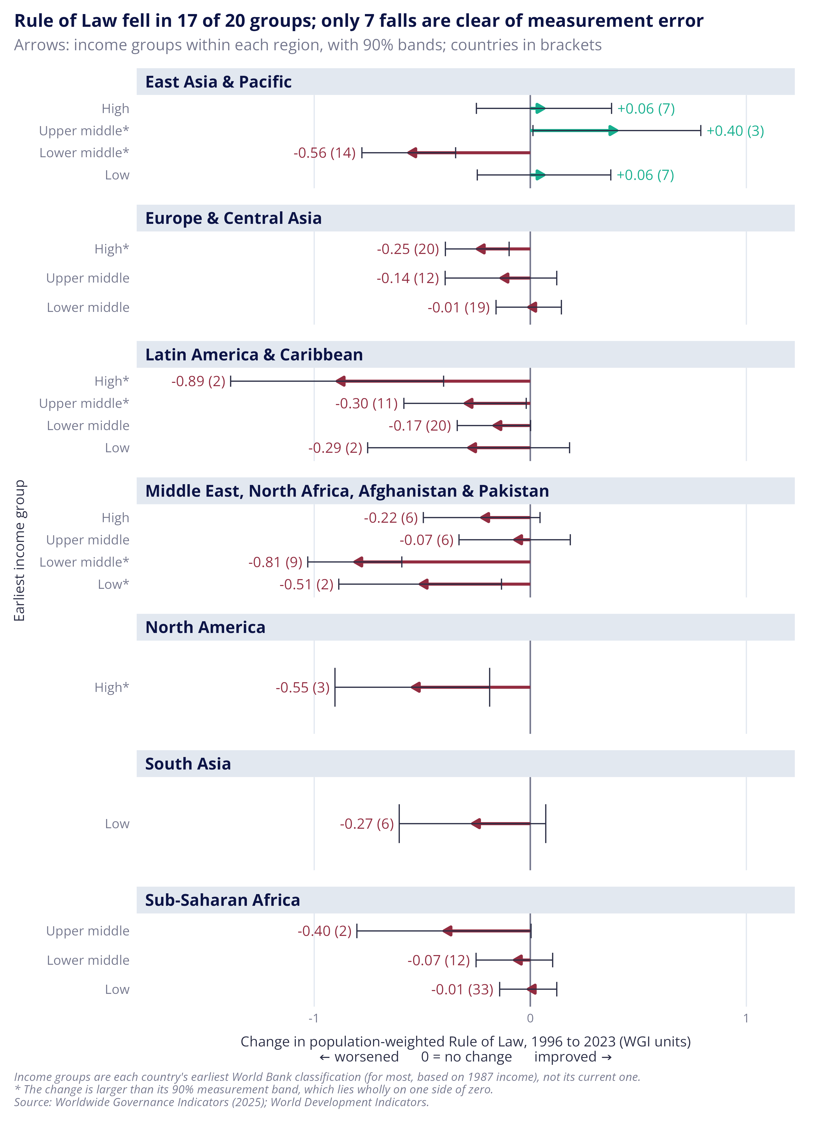
To get a sense of just how global these global averages are, the next figure presents average population-weighted score changes by region and income classification from 1996 to 2023. Each panel is a region and each arrow is an income group within it. The thin line over each arrow is the 90% measurement error band. Error bands crossing zero point to the direction of change in the rule of law being ambiguous.
Overall, countries across almost all regional and income groups experienced declines in their rule of law scores. The exception to this was in East Asia and the Pacific, where three income groups improved, though only one by more than the measurement error bands: the upper middle income group of South Korea, Macao and Palau. The general declines also line up with analysis by the World Justice Project, which found that countries with declines in their rule of law scores outnumbered those with improvements for nine years in a row.4
Note: A population-weighted decline doesn’t mean most countries got worse as more populous countries might be driving it (such as India in the chart above).
Figure: Change in population-weighted Rule of Law by starting income group within each region, 1996 to 2023
Code: plot-arrows-region-income
The code below calculates the population-weighted average for each income group within each region, in 1996 and 2023, and plots the change with a 90% measurement band. It also counts the falls that are clear of their band.
|
1 2 3 4 5 6 7 8 9 10 11 12 13 14 15 16 17 18 19 20 21 22 23 24 25 26 27 28 29 30 31 32 33 34 35 36 37 38 39 40 41 42 43 44 45 46 47 48 49 50 51 52 53 54 55 56 57 58 59 60 61 62 63 64 65 66 67 68 69 70 71 72 73 74 75 76 77 78 79 80 81 82 |
# Step 1: the population-weighted average for each group in each year, with its # standard error, worked out as for the world line above sum_region_income <- dta_panel_1996 |> summarise(wgi_rol_popw = weighted.mean(wgi_rol, w = pop_tot_nmb), wgi_rol_popw_se = sqrt(sum((pop_tot_nmb / sum(pop_tot_nmb))^2 * wgi_rol_se^2)), nmb_countries = n(), .by = c(region, econ_income_start, year)) # Step 2: copy each group's 1996 average and standard error onto its other # years, then keep 2023 only, leaving one line per group sum_region_income <- sum_region_income |> mutate(wgi_rol_popw_start = wgi_rol_popw[year == ref_year$start], wgi_rol_popw_se_start = wgi_rol_popw_se[year == ref_year$start], .by = c(region, econ_income_start)) |> filter(year == ref_year$end) # Step 3: the change since 1996 and its 90% band. The standard error of the # change combines the 1996 and 2023 errors, treating them as independent. sum_region_income <- sum_region_income |> mutate(wgi_rol_change = wgi_rol_popw - wgi_rol_popw_start, wgi_rol_change_se = sqrt(wgi_rol_popw_se^2 + wgi_rol_popw_se_start^2), change_low = wgi_rol_change - 1.645 * wgi_rol_change_se, change_high = wgi_rol_change + 1.645 * wgi_rol_change_se) # Step 4: colour and labels for the chart sum_region_income <- sum_region_income |> mutate(direction = if_else(wgi_rol_change < 0, "Decline", "Improvement"), # the short income group name (e.g. "Lower middle"), keeping the poorest-first order econ_income_short = fct_relabel(econ_income_start, \(x) unname(lkp_income$short[x]))) # The axis label: the short income group name, with an asterisk when the # whole 90% band lies on one side of zero. The labels are ordered poorest # first, as the income groups are. sum_region_income <- sum_region_income |> mutate(clear_of_error = change_high < 0 | change_low > 0, econ_income_label = paste0(econ_income_short, if_else(clear_of_error, "*", "")), econ_income_label = fct_reorder(econ_income_label, as.integer(econ_income_short))) # Falls whose whole 90% band lies below zero, counted in the chart title sum_region_income_clear <- sum_region_income |> filter(change_high < 0) plt_region_income <- sum_region_income |> ggplot(aes(y = econ_income_label, colour = direction)) + geom_vline(xintercept = 0, colour = ref_col$grey) + # every arrow starts at zero, so only the direction and size of the change show geom_segment(aes(x = 0, xend = wgi_rol_change, yend = econ_income_label), arrow = arrow(length = unit(0.2, "cm"), type = "closed"), linewidth = 1) + # 90% measurement band around each change, drawn on top of the arrow in dark # grey so both end ticks stay visible, including the one nearest zero geom_errorbar(aes(xmin = change_low, xmax = change_high), width = 0.5, colour = ref_col$charcoal, linewidth = 0.4) + # The label sits beyond the end of the band, on the side the arrow points. # The bracketed count shows how many countries sit behind each arrow. geom_text(aes(x = if_else(direction == "Decline", change_low, change_high), label = sprintf("%+.2f (%d)", wgi_rol_change, nmb_countries), hjust = if_else(direction == "Decline", 1.1, -0.1)), size = 3.6) + # free_y drops income groups a region doesn't have facet_wrap(~ region, ncol = 1, scales = "free_y") + scale_colour_manual(values = ref_col$direction) + scale_x_continuous(expand = expansion(mult = 0.2)) + # a shaded strip above each panel marks where one region ends and the next begins theme(legend.position = "none", axis.text.y = element_text(size = rel(1.05)), strip.text = element_text(size = rel(1.05), margin = margin(4, 6, 4, 6)), strip.background = element_rect(fill = ref_col$grey_pale, colour = NA), panel.spacing.y = unit(0.8, "lines"), panel.grid.major.y = element_blank(), panel.grid.major.x = element_line(colour = ref_col$grey_pale, linewidth = 0.4)) + labs(title = sprintf("Rule of Law fell in %d of %d groups; only %d falls are clear of measurement error", sum(sum_region_income$direction == "Decline"), nrow(sum_region_income), nrow(sum_region_income_clear)), subtitle = "Arrows: income groups within each region, with 90% bands; countries in brackets", x = paste0("Change in population-weighted Rule of Law, 1996 to 2023 (WGI units)\n", ref_lab$axis_change), y = "Earliest income group", caption = paste(ref_lab$income_start, ref_lab$clear_of_error, ref_lab$caption, sep = "\n")) plt_region_income |
Countries with stronger rule of law are richer
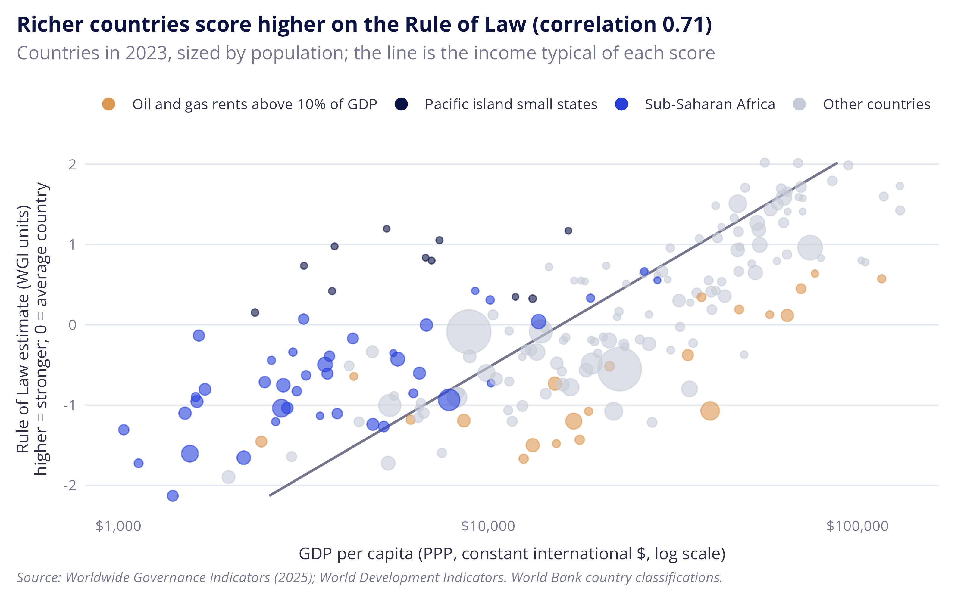
You don’t need to be an economist to guess that the rule of law is probably stronger in richer countries5, but scatter plots demonstrating this appear in almost every governance report talking about the rule of law. The plot below demonstrates this by comparing each country’s rule of law score in 2023 with its GDP per capita. Purchasing power parity (PPP) terms are used to adjust for differences in purchasing power, such that one PPP dollar has the same real value across countries.
The line on the plot shows the typical relationship between the rule of law and average income. Countries to the left of the line are poorer than might be expected given their rule of law scores, while those to the right of the line are wealthier. Although why countries sit on either side is a rabbit hole worth exploring, a large share of the outliers can be explained by geography and the structure of a country’s economy, in particular:
- Countries that are wealthier than might be expected given their rule of law score: include economies that rely heavily on oil and gas rents, which is theorised to reduce the incentive for government to create inclusive institutions for the benefit of the wider public.6
- Countries that are poorer than might be expected given their rule of law score: include a large share of Pacific island economies and countries in Sub-Saharan Africa. While the reasons are beyond the scope of this post, Pacific island economies are unusually small and remote, depressing economic activity and trade, while many of the countries in Sub-Saharan Africa face wider institutional and geographic challenges, such as poor governance and having a smaller share of their population near navigable rivers.7
As always, my point here isn’t to imply the two things are causally connected as the claim requires more evidence than a pairwise correlation. But, the idea that more secure, predictable and legible property rights might make trade and commerce easier isn’t new, which means there’s plenty of evidence exploring the idea.8 It’s also a compelling idea to anybody who has spent their career being inundated with governance reports presenting the correlation.
But, there’s also an arguable conceptual endogeneity9 between GDP per capita and the rule of law. The rule of law plays a central role in deciding what can be owned, priced and traded, while also being shaped by the same political and economic forces it is meant to govern.10 So by strengthening the rule of law, what can be owned, priced and traded changes too,11 thereby expanding what can be counted in GDP statistics. That doesn’t make the connection meaningless as GDP is connected with other things we care about like life expectancy and wellbeing. But it’s good to keep in mind as it’s likely that some part of the correlation reflects their overlapping and mutually reinforcing scope, rather than simply being a clean relationship between two independent variables.
Note: Oil and gas rents are the value of oil and gas production less what it costs to extract, as a share of GDP, from the World Development Indicators.
Code: levels-data
The code below produces a scatter plot comparing a country’s rule of law score with GDP per capita in 2023. The size of each country’s point is scaled by population, while economies with significant oil rents (>10%), Pacific island small states and Sub-Saharan African countries are coloured.
|
1 2 3 4 5 6 7 8 9 10 11 12 13 14 15 16 17 18 19 20 21 22 23 24 25 26 27 28 29 30 31 32 33 34 35 36 37 38 39 40 41 42 43 44 45 46 47 48 49 50 51 52 53 54 55 56 57 |
# Every country with a score and an income in 2023 dta_rol_income <- dta_panel |> filter(year == ref_year$end, !is.na(wgi_rol), !is.na(econ_gdppc_ppp)) # Correlation between the score and log income, for the chart title sum_cor_rol_income <- cor(dta_rol_income$wgi_rol, log(dta_rol_income$econ_gdppc_ppp)) # Oil and gas rents for each country, averaged over 2019 to 2023 because they # swing with prices. Countries with no rents data get NaN (not a number). dta_oilgas_rents <- dta_panel |> filter(year %in% ref_year$rents_window) |> summarise(res_oilgas_pct = mean(res_oil_rents_pct + res_gas_rents_pct, na.rm = TRUE), .by = iso3c) # The World Bank's Pacific island small states (group PSS), taken from the # "composition" sheet of its CLASS workbook, downloaded 7 November 2026 ref_pacific_islands <- read_csv(ref_path$pacific, show_col_types = FALSE) dta_rol_income <- dta_rol_income |> left_join(dta_oilgas_rents, by = join_by(iso3c), relationship = "one-to-one") # The colour group of each country on the chart. case_when() takes the first rule # that is true, so an African producer counts as a producer. Countries with no # rents data are not producers. dta_rol_income <- dta_rol_income |> mutate(point_group = case_when( res_oilgas_pct > ref_cutoff$large_producer_rents_pct ~ ref_lab$large_producers, iso3c %in% ref_pacific_islands$iso3c ~ "Pacific island small states", region == "Sub-Saharan Africa" ~ "Sub-Saharan Africa", .default = "Other countries")) # The colour of each group on the chart; this order is also the legend order lkp_point_colours <- c(ref_col$orange, ref_col$navy, ref_col$blue, ref_col$grey_light) names(lkp_point_colours) <- c(ref_lab$large_producers, "Pacific island small states", "Sub-Saharan Africa", "Other countries") plt_rol_income <- dta_rol_income |> ggplot(aes(x = econ_gdppc_ppp, y = wgi_rol)) + # a straight line of log income on the score; orientation = "y" fits income on the # score, so a country to the right of the line is richer than its score suggests geom_smooth(method = "lm", formula = y ~ x, orientation = "y", se = FALSE, colour = ref_col$grey, linewidth = 0.7) + geom_point(aes(size = pop_tot_nmb, colour = point_group), alpha = 0.6) + scale_x_log10(labels = scales::label_dollar()) + scale_colour_manual(values = lkp_point_colours, breaks = names(lkp_point_colours)) + guides(colour = guide_legend(override.aes = list(size = 3, alpha = 1))) + # a minimum point size keeps the smallest countries, such as the Pacific islands, visible scale_size(range = c(1.5, 12), guide = "none") + labs(title = sprintf("Richer countries score higher on the Rule of Law (correlation %.2f)", sum_cor_rol_income), subtitle = paste0("Countries in ", ref_year$end, ", sized by population; the line is the income typical of each score"), x = "GDP per capita (PPP, constant international $, log scale)", y = paste0("Rule of Law estimate (WGI units)\n", ref_lab$axis_score_vertical), caption = paste(ref_lab$caption, "World Bank country classifications.")) plt_rol_income |
But economic growth without the rule of law exists
Almost every discussion of the links between institutions and economic growth eventually turns to China. China, so the story goes, has grown quickly without investing in pesky institutions like the rule of law.12 This section tests that story in two steps: first by comparing growth with where countries started on the rule of law in 1996, and then by comparing growth with how their rule of law changed over the period.
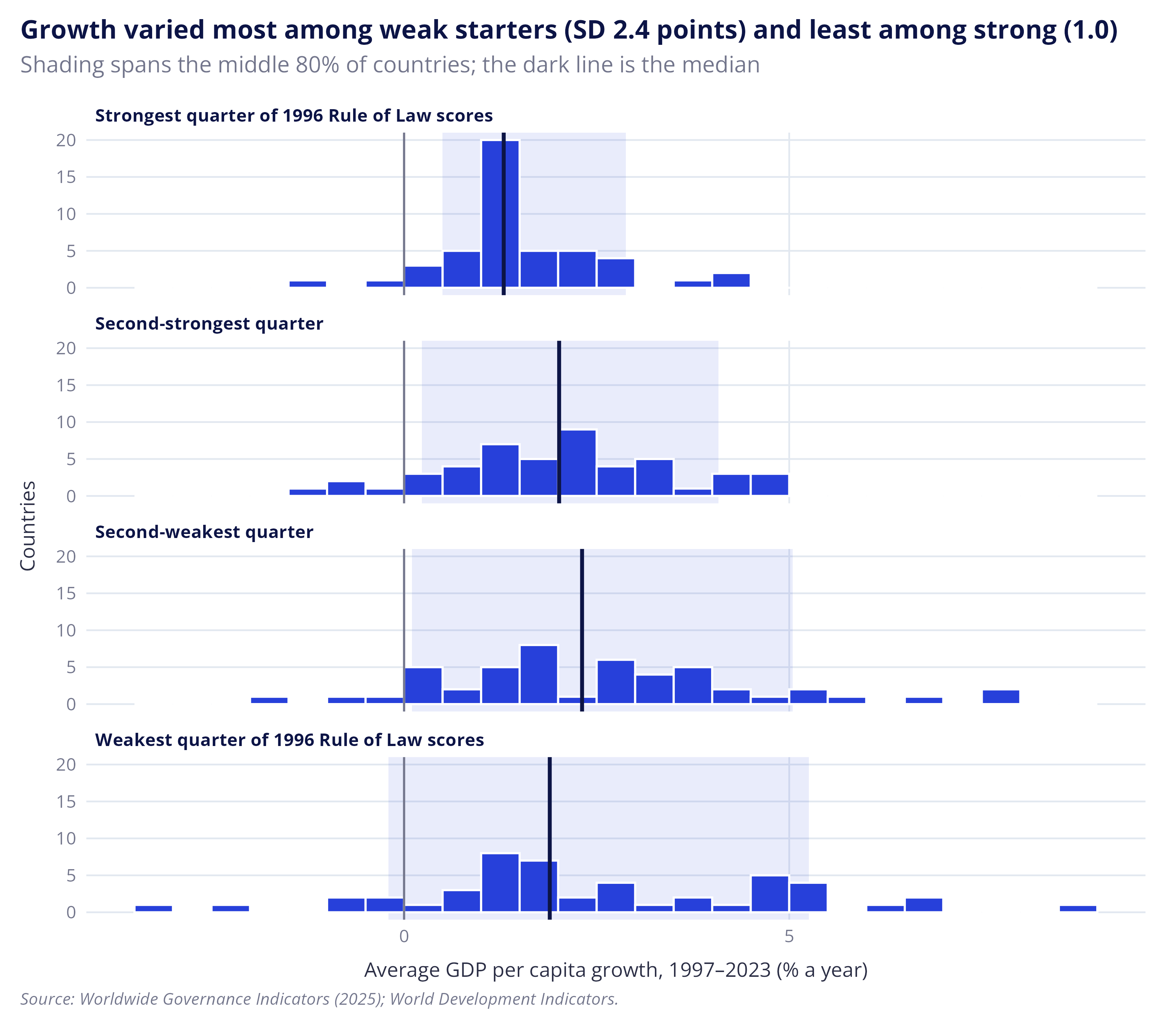
The plot below shows the distribution of average GDP per capita growth from 1997 to 2023, with countries grouped into four groups based on their rule of law score in 1996. It’s as good a time as any to repeat the warning about drawing sweeping conclusions from observational analysis like this, but the data suggests two things about economic growth and the rule of law:
- Strong growth is possible where the rule of law is weak: many of the countries that started with weak scores grew faster than those that started with strong ones; and
- A strong rule of law doesn’t guarantee high growth: the countries with the strongest rule of law scores in 1996 had the lowest median growth of the four groups.13
Note: Most of the countries in the strongest quarter were already high income at the start of the period, and richer countries tend to grow more slowly, partly because they have less room to catch up.
Figure: Average growth 1997–2023 by Rule of Law in 1996
Code: plot-growth-vs-start
The code below calculates the average annual economic growth and presents this as a histogram with countries grouped according to their rule of law score in 1996.
|
1 2 3 4 5 6 7 8 9 10 11 12 13 14 15 16 17 18 19 20 21 22 23 24 25 26 27 28 29 30 31 32 33 34 35 36 37 38 39 40 41 42 43 44 45 46 |
# One line per country: its score in 1996 and 2023, and its average growth. # Growth in 1996 itself happened before the starting score, so it is left out. # first() returns the single value for that year, or NA if the country has none. # Some countries miss a few years of growth, hence na.rm = TRUE. dta_country_growth <- dta_panel |> summarise( wgi_rol_start = first(wgi_rol[year == ref_year$start]), wgi_rol_end = first(wgi_rol[year == ref_year$end]), wgi_rol_se_start = first(wgi_rol_se[year == ref_year$start]), wgi_rol_se_end = first(wgi_rol_se[year == ref_year$end]), econ_growth_avg_pct = mean(econ_gdppc_growth_pct[year > ref_year$start], na.rm = TRUE), nmb_growth_years = sum(!is.na(econ_gdppc_growth_pct[year > ref_year$start])), .by = c(iso3c, country, region)) # Keep countries with a 1996 score and at least 20 years of growth data, then # add the change in score and the starting income group dta_country_growth <- dta_country_growth |> filter(!is.na(wgi_rol_start), nmb_growth_years >= ref_cutoff$min_growth_years) |> mutate(wgi_rol_change = wgi_rol_end - wgi_rol_start) |> left_join(lkp_income_start, by = join_by(iso3c), relationship = "one-to-one") # Panel titles, weakest starting score first lkp_quarter_titles <- c("Weakest quarter of 1996 Rule of Law scores", "Second-weakest quarter", "Second-strongest quarter", "Strongest quarter of 1996 Rule of Law scores") # ntile() splits the countries into four equal-sized groups by their 1996 score, # 1 being the weakest. rev() reverses the panel order only, so the strongest # quarter is drawn at the top. dta_country_growth <- dta_country_growth |> mutate(start_quarter = ntile(wgi_rol_start, 4), start_quarter_label = factor(lkp_quarter_titles[start_quarter], levels = rev(lkp_quarter_titles))) # Median, spread and counts for each quarter, used in the chart and the note # above it (how many in each quarter started as high income) sum_growth_quarter <- dta_country_growth |> summarise(nmb_countries = n(), nmb_high_income = sum(econ_hic_start == "High income"), growth_median = median(econ_growth_avg_pct), growth_sd = sd(econ_growth_avg_pct), growth_p10 = quantile(econ_growth_avg_pct, 0.1), growth_p90 = quantile(econ_growth_avg_pct, 0.9), .by = c(start_quarter, start_quarter_label)) |> arrange(start_quarter) sum_growth_quarter |
# A tibble: 4 × 8
  start_quarter start_quarter_label  nmb_countries nmb_high_income growth_median
          <int> <fct>                        <int>           <int>         <dbl>
1             1 Weakest quarter of …            48               0          1.89
2             2 Second-weakest quar…            48               0          2.31
3             3 Second-strongest qu…            48               5          2.01
4             4 Strongest quarter o…            47              31          1.29
# ℹ 3 more variables: growth_sd <dbl>, growth_p10 <dbl>, growth_p90 <dbl>
|
1 2 3 4 5 6 7 8 9 10 11 12 13 14 15 16 17 18 19 20 |
plt_growth_quarter <- dta_country_growth |> ggplot(aes(x = econ_growth_avg_pct)) + # shaded band: the middle 80% of countries in each quarter geom_rect(data = sum_growth_quarter, inherit.aes = FALSE, aes(xmin = growth_p10, xmax = growth_p90, ymin = -Inf, ymax = Inf), fill = ref_col$blue, alpha = 0.1) + geom_histogram(binwidth = 0.5, boundary = 0, fill = ref_col$blue, colour = "white") + geom_vline(xintercept = 0, colour = ref_col$grey) + # the median of each quarter geom_vline(data = sum_growth_quarter, aes(xintercept = growth_median), colour = ref_col$navy, linewidth = 0.9) + facet_wrap(~ start_quarter_label, ncol = 1) + theme(panel.grid.major.x = element_line(colour = ref_col$grey_pale, linewidth = 0.4)) + labs(title = sprintf("Growth varied most among weak starters (SD %.1f points) and least among strong (%.1f)", sum_growth_quarter$growth_sd[1], sum_growth_quarter$growth_sd[4]), subtitle = "Shading spans the middle 80% of countries; the dark line is the median", x = "Average GDP per capita growth, 1997–2023 (% a year)", y = "Countries", caption = ref_lab$caption) plt_growth_quarter |
Countries where the rule of law improved were more likely to grow faster
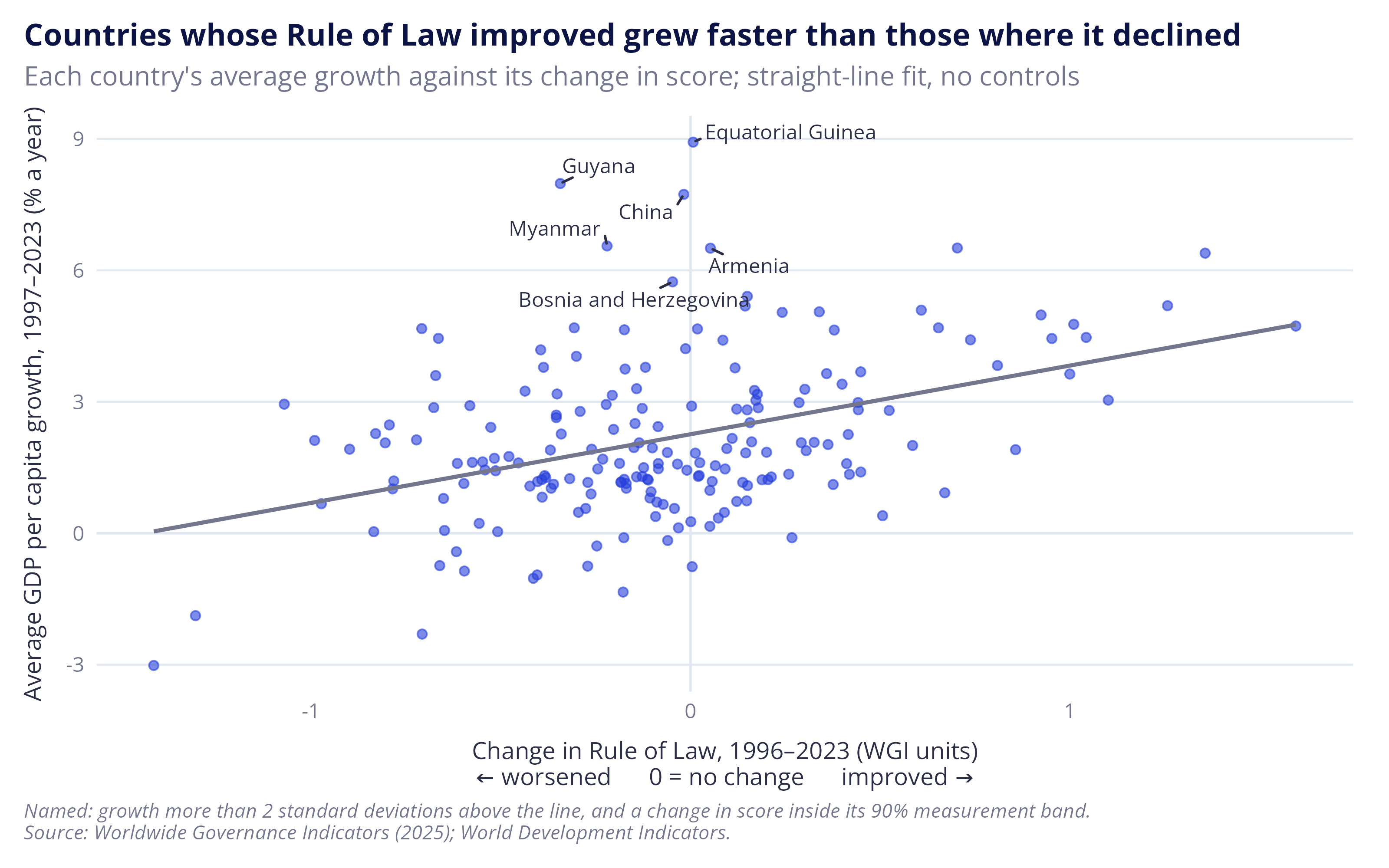
The histogram above looked at growth against a country’s level of rule of law in 1996. The plot below looks at growth against the change in its rule of law score between 1996 and 2023.
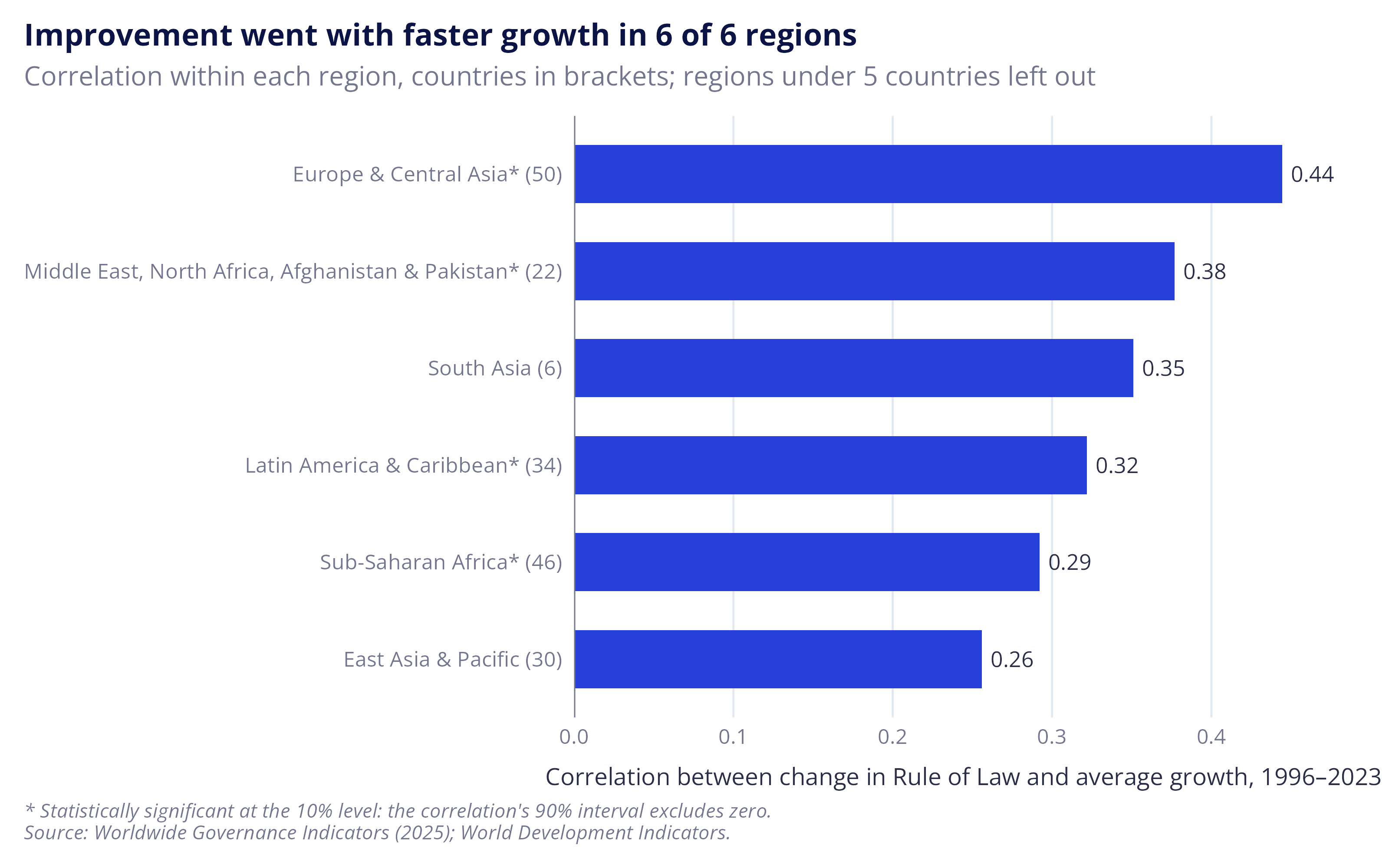
In essence, it asks whether countries whose rule of law improved more also grew faster. The answer is a qualified yes, and the relationship is positive in every region with enough countries to measure it.
This isn’t to say that improvements in the rule of law cause economic growth14, only that the two have moved together over the last three decades. Causality could run the other way, with faster-growing countries able to spend more on the courts, police and other systems that support the rule of law, or it could run both ways. Other drivers of growth may also be missing from the analysis, such as the quality of regulation and political accountability, which are closely tied to the rule of law. Even so, the pattern helps explain why economists are so excited to talk about how and why the two might be linked.
The plot also highlights countries that grew faster than might be expected given changes in their score. China, the example that everyone raises, is there but isn’t alone: Equatorial Guinea, Guyana, Myanmar, Armenia, and Bosnia and Herzegovina all sit well above the line with no clear change in their rule of law score. Several have likely explanations, such as oil discoveries, economic recovery after war and the breakdown of the Soviet Union. China’s small change over the period also hides a fall in its score in the mid-2000s which was followed by a long recovery. None of this is to deny that China holds lessons about institutions and growth (it does), only that it’s not the only outlier that’s worth explaining.
Note: North America showed the opposite relationship but is left off the regional chart, as it has only three countries (Bermuda, Canada and the United States).
Figures: Change in Rule of Law and average growth, 1996–2023, for all countries and by region
Code: plot-growth-vs-change
The code below produces two plots: a scatter plot comparing economic growth with changes in the rule of law, with the unusually fast growers whose score didn’t clearly change named, and a bar plot that reports the correlation between the two variables within each region.
|
1 2 3 4 5 6 7 8 9 10 11 12 13 14 15 16 17 18 19 20 21 22 23 24 25 26 27 28 29 30 31 32 33 34 35 36 37 38 39 40 |
# The countries in the histograms that have a score in 2023 as well as 1996 dta_growth_change <- dta_country_growth |> filter(!is.na(wgi_rol_change)) # How far each country's growth sits above or below the straight line drawn # through all countries, in percentage points dta_growth_change <- dta_growth_change |> mutate(growth_vs_line = residuals(lm(econ_growth_avg_pct ~ wgi_rol_change))) # The countries named on the chart: growth more than two standard deviations # of these distances above the line, and a change in score inside its 90% # measurement band, worked out as for the five most populous countries dta_growth_change <- dta_growth_change |> mutate(wgi_rol_change_se = sqrt(wgi_rol_se_start^2 + wgi_rol_se_end^2), change_within_band = abs(wgi_rol_change) <= 1.645 * wgi_rol_change_se, fast_no_change = growth_vs_line > ref_cutoff$outlier_sd * sd(growth_vs_line) & change_within_band) plt_growth_change <- dta_growth_change |> ggplot(aes(x = wgi_rol_change, y = econ_growth_avg_pct)) + geom_hline(yintercept = 0, colour = ref_col$grey_pale) + geom_vline(xintercept = 0, colour = ref_col$grey_pale) + geom_point(colour = ref_col$blue, alpha = 0.6) + # one straight-line fit through all countries, with no controls geom_smooth(method = "lm", formula = y ~ x, se = FALSE, colour = ref_col$grey, linewidth = 0.8) + # name the fast growers whose score didn't clearly change, China among them. # Each label is joined to its point by a short line (min.segment.length = 0 always draws it). geom_text_repel(data = filter(dta_growth_change, fast_no_change), aes(label = country), size = 3, colour = ref_col$charcoal, family = "Open Sans", seed = 1, min.segment.length = 0) + labs(title = "Countries whose Rule of Law improved grew faster than those where it declined", subtitle = "Each country's average growth against its change in score; straight-line fit, no controls", x = paste0("Change in Rule of Law, 1996–2023 (WGI units)\n", ref_lab$axis_change), y = "Average GDP per capita growth, 1997–2023 (% a year)", caption = paste(sprintf("Named: growth more than %d standard deviations above the line, and a change in score inside its 90%% measurement band.", ref_cutoff$outlier_sd), ref_lab$caption, sep = "\n")) plt_growth_change |
|
1 2 3 4 5 6 7 8 9 10 11 12 13 |
# Correlation between the change in score and average growth within each region sum_cor_region <- dta_growth_change |> summarise(nmb_countries = n(), cor_change = cor(wgi_rol_change, econ_growth_avg_pct), .by = region) # Regions with fewer countries than the cut-off are left off the chart. On the # data used here (checked 10 November 2026) this is North America (3 countries: # Bermuda, Canada and the United States). sum_cor_small_regions <- sum_cor_region |> filter(nmb_countries < ref_cutoff$min_group_countries) sum_cor_small_regions |
# A tibble: 1 × 3
  region        nmb_countries cor_change
  <chr>                 <int>      <dbl>
1 North America             3     -0.943
|
1 2 3 4 5 6 7 8 9 10 11 12 13 14 15 16 17 18 19 20 21 22 23 24 25 26 27 28 29 30 31 32 33 34 35 36 37 38 39 40 |
# Keep the regions large enough to chart sum_cor_region <- sum_cor_region |> filter(nmb_countries >= ref_cutoff$min_group_countries) # Is each correlation statistically significant at the 10% level, matching the # 90% bands used elsewhere in the post? This is the standard test that the # correlation is zero, written out: the t statistic is # r x sqrt((n - 2) / (1 - r^2)), with n - 2 degrees of freedom. It gives the # same p-value as cor.test(). sum_cor_region <- sum_cor_region |> mutate(cor_t = cor_change * sqrt((nmb_countries - 2) / (1 - cor_change^2)), cor_p_value = 2 * pt(-abs(cor_t), df = nmb_countries - 2), cor_signif = cor_p_value < 0.10) # The labels: an asterisk after the region when the correlation is significant, # and the number of countries in brackets sum_cor_region <- sum_cor_region |> mutate(region_label = sprintf("%s%s (%d)", region, if_else(cor_signif, "*", ""), nmb_countries), # largest correlation at the top region_label = fct_reorder(region_label, cor_change)) plt_cor_region <- sum_cor_region |> ggplot(aes(x = cor_change, y = region_label)) + geom_col(fill = ref_col$blue, width = 0.6) + geom_vline(xintercept = 0, colour = ref_col$grey) + # the value sits just beyond the end of each bar geom_text(aes(label = sprintf("%.2f", cor_change)), hjust = -0.2, size = 3.2) + scale_x_continuous(expand = expansion(mult = c(0, 0.1))) + theme(panel.grid.major.y = element_blank(), panel.grid.major.x = element_line(colour = ref_col$grey_pale, linewidth = 0.4)) + labs(title = sprintf("Improvement went with faster growth in %d of %d regions", sum(sum_cor_region$cor_change > 0), nrow(sum_cor_region)), subtitle = sprintf("Correlation within each region, countries in brackets; regions under %d countries left out", ref_cutoff$min_group_countries), x = "Correlation between change in Rule of Law and average growth, 1996–2023", y = NULL, caption = paste("* Statistically significant at the 10% level: the correlation's 90% interval excludes zero.", ref_lab$caption, sep = "\n")) plt_cor_region |
Summing up
The point of this post, besides satisfying my curiosity about the data, was to lay out a set of common themes that emerge in the literature:
- Globally, the rule of law has deteriorated since the mid 90s;
- The rule of law and economic growth appear to be linked;
- The rule of law’s relationship with economic growth is positive across regions; and
- The rule of law isn’t a necessary or sufficient condition for economic growth.
If you’re familiar with the field, none of this will be particularly surprising, but each of these themes provides useful context for future posts where I attempt to tease out some of these relationships and trends in greater detail. But, I also wanted to make a contribution to the grey literature on the topic as from my observations there are few explorations of the topic that dig into the technical details outside published papers on the topic.
World Bank (2025). “The Worldwide Governance Indicators: revised methodology for measuring governance using perception data.” December 2025. Prepared by C. N. Jiang, A. Jain, T. Romano and T. Boyce.↩︎
Gallup, J. L., Sachs, J. D. and Mellinger, A. D. (1999). “Geography and economic development.” International Regional Science Review 22(2): 179–232.↩︎
Kaufmann, D., Kraay, A. and Mastruzzi, M. (2010). “The Worldwide Governance Indicators: methodology and analytical issues.” World Bank Policy Research Working Paper 5430.↩︎
World Justice Project (2026). WJP Rule of Law Index 2026. Washington, DC: World Justice Project. Released 21 October 2026. worldjusticeproject.org/rule-of-law-index↩︎
Analysis also points to the correlation becoming stronger over time, see: Bhagat, S., 2020. Economic growth, income inequality, and the rule of law. Harvard Business Law Review Online.↩︎
Natural Resource Governance Institute 2015, The resource curse: The political and economic challenges of natural resource wealth , NRGI Reader, viewed 7 November 2026, resourcegovernance.org.↩︎
Distance from the sea and access to inland rivers may also play a part. Countries where fewer than a quarter of people live within 100 km of a coast or navigable river are mostly poorer than their score predicts (many of them are in Sub-Saharan Africa). I tested this using Gallup, Sachs and Mellinger’s geography data (RePEc), but left the analysis and grouping off the chart as it largely picks out countries in Sub-Saharan Africa and I didn’t want to imply there was a simple explanation for something this complicated. In my defence, I’m in good company: Adam Smith argued that water transport widens markets and Jeffrey Sachs and co-authors make a similar case for navigable water, see: Mellinger, A.D., Sachs, J.D. and Gallup, J.L., 1999. Climate, water navigability, and economic development. CID Working Paper No. 24, Center for International Development, Harvard University.↩︎
For instance, see: Rigobon, R. and Rodrik, D., 2005. Rule of law, democracy, openness, and income: Estimating the interrelationships. Economics of transition, 13(3), pp.533-564; Haggard, S. and Tiede, L., 2011. The rule of law and economic growth: where are we?. World development, 39(5), pp.673-685; and Butkiewicz, J.L. and Yanikkaya, H., 2006. Institutional quality and economic growth: Maintenance of the rule of law or democratic institutions, or both?. Economic Modelling, 23(4), pp.648-661.↩︎
In addition to the statistical endogeneity, such as wealthier nations being more able to invest in their legal and regulatory systems.↩︎
e.g. see: Krever, T., 2011. The legal turn in late development theory: The rule of law and the World Bank’s development model. Harv. Int’l LJ, 52, p.287; and Haggard, S., MacIntyre, A. and Tiede, L., 2008. The rule of law and economic development. Annu. Rev. Polit. Sci., 11(1), pp.205-234.↩︎
Pistor makes a similar point in her book ‘The Code of Capital’, noting that: the law allows the attachment of “…wealth generating attributes, namely priority, durability, convertibility, and universality onto different assets.” See: Pistor, K., 2019. The code of capital: How the law creates wealth and inequality. Princeton University Press.↩︎
For a good overview of why it’s thought China has achieved this, see: Lopez-Gomez, L. (2026) The Rule of Law and the Institutional Roots of Economic Performance: Literature Review. London: Bingham Centre for the Rule of Law and the Law Society of England and Wales. Available at: https://binghamcentre.biicl.org/publications/the-rule-of-law-and-the-institutional-roots-of-economic-performance, p.17↩︎
The non-linear relationship between the rule of law and other institutional variables is well-documented, e.g. Beyaert, A., García-Solanes, J. and Lopez-Gomez, L., 2023. Corruption, quality of institutions and growth. Applied economic analysis, 31(91), pp.55-72.↩︎
This isn’t to say evidence doesn’t exist: for instance, Besley et al. (2025) found that areas in England with greater legal capacity during the industrial revolution achieved better social, economic and institutional outcomes. Because it’s plausible that legal capacity has been exogenously determined, the authors believe the association can be interpreted as being causal. See: Besley, T., Bogart, D., Chapman, J. and Palma, N., 2025. Justices of the peace: Legal foundations of the industrial revolution (No. 20214). Centre for Economic Policy Research.↩︎